Utility Theory Notes: Cardinal vs Ordinal, Marginal Utility, Law of DMU & Demand Curve Derivation
Comprehensive notes on Utility Theory: Cardinal vs Ordinal approaches, Law of Diminishing Marginal Utility, indifference curves, and demand curve derivation.
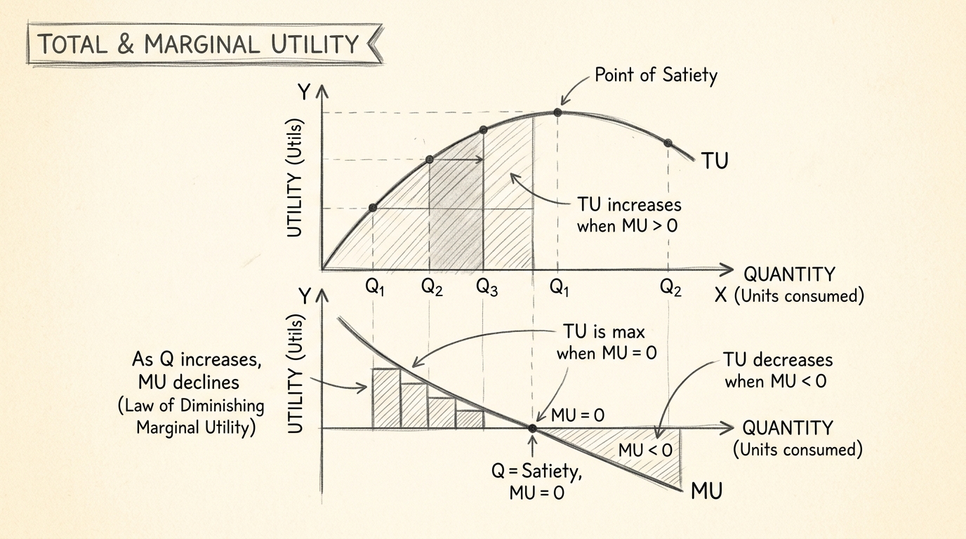
Why do consumers buy what they buy? How do they allocate their limited income across a vast array of goods to maximize satisfaction? These are the foundational questions of Consumer Behavior theory. To answer them, economists developed Utility Theory. This article breaks down both the classic Cardinal approach (Alfred Marshall) and the modern Ordinal approach (J.R. Hicks and R.G.D. Allen), explains the laws governing them, derives the demand curve, and includes robust numerical problems.
1. The Cardinal Utility Approach (Marshallian)
The Cardinal Utility approach assumes that utility (satisfaction) is a measurable entity. According to Marshall, we can measure utility in absolute quantitative units called "utils".
Key Concepts
- Total Utility (TU): The total satisfaction derived from consuming a given quantity of a good.
- Marginal Utility (MU): The additional satisfaction derived from consuming one more unit of a good. Mathematically, MU = d(TU)/dQ.
The Law of Diminishing Marginal Utility (DMU)
This law states that as a consumer consumes more and more units of a specific commodity, the marginal utility derived from each successive unit goes on diminishing.
Relationship between TU and MU:
1. When MU is positive, TU is increasing.
2. When MU is zero, TU is at its maximum (Point of Satiation).
3. When MU becomes negative, TU starts declining.
Exceptions to DMU: Hobbies/Collections (stamp collecting), Money/Wealth (greed), and intoxicants (addiction). However, these are strictly debated in pure theory.
Consumer Equilibrium (Equi-Marginal Principle)
A rational consumer aims to maximize total utility subject to their budget constraint.
For a single good: Equilibrium is achieved when MUx = Px (assuming marginal utility of money is 1).
For two goods (x and y): Equilibrium is achieved when the ratio of marginal utility to price is equal across goods:
MUx / Px = MUy / Py = MUm
Derivation of the Demand Curve
The downward-sloping demand curve is a direct consequence of the Law of DMU. Because successive units yield less utility, a consumer is only willing to buy additional units if the price is lower. Thus, Price must equal Marginal Utility (P = MU). As Q increases, MU falls; therefore, P must fall to induce the consumer to buy more, resulting in a downward-sloping demand curve.
2. The Ordinal Utility Approach (Hicks-Allen)
Economists realized that psychological satisfaction cannot be quantified in absolute "utils". Hicks and Allen introduced Ordinal Utility, suggesting consumers can only rank their preferences (1st, 2nd, 3rd) rather than measure them exactly.
Preference Axioms
- Completeness: For any bundles A and B, the consumer either prefers A to B, prefers B to A, or is indifferent between them.
- Transitivity: If A is preferred to B, and B is preferred to C, then A must be preferred to C.
- Non-satiation (More is better): A bundle with more of at least one good and no less of any other is strictly preferred.
Indifference Curves (IC)
An Indifference Curve represents all combinations of two goods (X and Y) that yield the exact same level of total satisfaction to the consumer.
Properties of ICs:
1. Downward sloping (due to non-satiation).
2. Convex to the origin (due to diminishing Marginal Rate of Substitution - MRS).
3. Higher IC represents higher utility.
4. ICs cannot intersect (violates transitivity).
Consumer Equilibrium in Ordinal Utility
Equilibrium occurs where the highest possible Indifference Curve is tangent to the Budget Line.
Budget Line equation: Px*X + Py*Y = M (Income)
Tangency Condition: MRSxy = Px / Py
(Since MRSxy = MUx / MUy, this mirrors the equi-marginal principle: MUx / MUy = Px / Py).
3. Cardinal vs Ordinal Comparison Table
| Feature | Cardinal Utility (Marshall) | Ordinal Utility (Hicks-Allen) |
|---|---|---|
| Measurability | Quantitative (Utils) | Qualitative (Ranking/Ordering) |
| Analytical Tool | Marginal Utility Analysis | Indifference Curve Analysis |
| Marginal Utility of Money | Assumed constant | Not assumed constant |
| Demand Analysis | Cannot separate Income & Substitution effects | Successfully decomposes Income & Substitution effects |
4. Marshallian vs Hicksian Demand
Marshallian Demand (Uncompensated): Demand derived holding nominal income constant. It incorporates both substitution and income effects.
Hicksian Demand (Compensated): Demand derived holding utility constant. It isolates the pure substitution effect. The Hicksian demand curve is always downward sloping, even for Giffen goods.
5. Consumer Surplus
The difference between what a consumer is willing to pay (based on utility) and what they actually pay (market price). Graphically, it is the area below the demand curve and above the price line.
6. Worked Numerical Problems
Problem 1: Equi-Marginal Principle
Question: Consumer has M = ₹40. Px = ₹10, Py = ₹5. MU schedules are:
Q: 1, 2, 3, 4
MUx: 50, 40, 30, 20
MUy: 30, 20, 15, 10
Find optimal consumption.
Solution:
Calculate MU/P for each:
MUx/Px: 50/10=5, 40/10=4, 30/10=3, 20/10=2
MUy/Py: 30/5=6, 20/5=4, 15/5=3, 10/5=2
Equate MUx/Px = MUy/Py.
Possibility A: MUx/Px = MUy/Py = 4. This happens at 2 units of X and 2 units of Y.
Check Budget: 10(2) + 5(2) = 20 + 10 = 30. (Doesn't exhaust ₹40).
Possibility B: MUx/Px = MUy/Py = 3. This happens at 3 units of X and 3 units of Y.
Check Budget: 10(3) + 5(3) = 30 + 15 = 45. (Exceeds ₹40 budget).
Wait, let's look for integer allocation: Buy 2 units of X (cost 20, MUx/Px=4) and 4 units of Y (cost 20, MUy/Py=2). Here MUx/Px ≠ MUy/Py.
Let's trace utility step by step:
Spend first ₹5: Buy Y (MU/P = 6). Total spent = 5.
Spend next ₹10: Buy X (MU/P = 5). Total spent = 15.
Spend next ₹5: Buy Y (MU/P = 4). Total spent = 20.
Spend next ₹10: Buy X (MU/P = 4). Total spent = 30.
Spend final ₹10: Buy 2 units of Y (MU/P = 3 and 2) or 1 unit of X (MU/P = 3).
Wait, if we buy 1 X, we get 30 utility for 10 rupees (3 per rupee). If we buy 2 Ys, we get 15+10=25 utility for 10 rupees (2.5 per rupee).
So, buy X.
Final bundle: 3 units of X, 2 units of Y. Total expenditure: 3(10) + 2(5) = 40.
Here, MUx/Px for 3rd unit = 3. MUy/Py for 2nd unit = 4. Marginal conditions are approximate due to lumpiness of goods.
Problem 2: Deriving Demand Function
Question: Utility function U(X,Y) = X^0.5 * Y^0.5. M = 100, Px = 2, Py = 4. Find X and Y.
Solution:
This is a Cobb-Douglas utility function. MUx = 0.5 * (Y/X)^0.5. MUy = 0.5 * (X/Y)^0.5.
MRSxy = MUx / MUy = Y / X.
Equilibrium condition: MRS = Px / Py => Y / X = 2 / 4 = 1/2 => X = 2Y.
Substitute into budget constraint: Px*X + Py*Y = M
2*(2Y) + 4*Y = 100 => 4Y + 4Y = 100 => 8Y = 100 => Y = 12.5.
X = 2Y = 25.
Optimal Bundle: X = 25, Y = 12.5.
Problem 3: Marginal Utility calculation
Question: TU = 100Q - 2Q^2. Find MU and the quantity where satiation is reached.
Solution:
MU = d(TU)/dQ = 100 - 4Q.
Satiation is reached when MU = 0.
100 - 4Q = 0 => 4Q = 100 => Q = 25.
Note for exams: Always state your assumptions clearly, particularly whether you are using Cardinal or Ordinal framework, and clearly label all axes and curves on your graphs.
Frequently asked questions
What is the equi-marginal principle?
Consumers maximize utility by equating the ratio of marginal utility to price across all goods consumed.
Why are indifference curves convex to the origin?
Due to the diminishing marginal rate of substitution between the two goods.
Dhairya sat the same DU papers he now writes about. Acadly is his attempt to say the useful things his own first-year self would have wanted to hear.
Keep reading
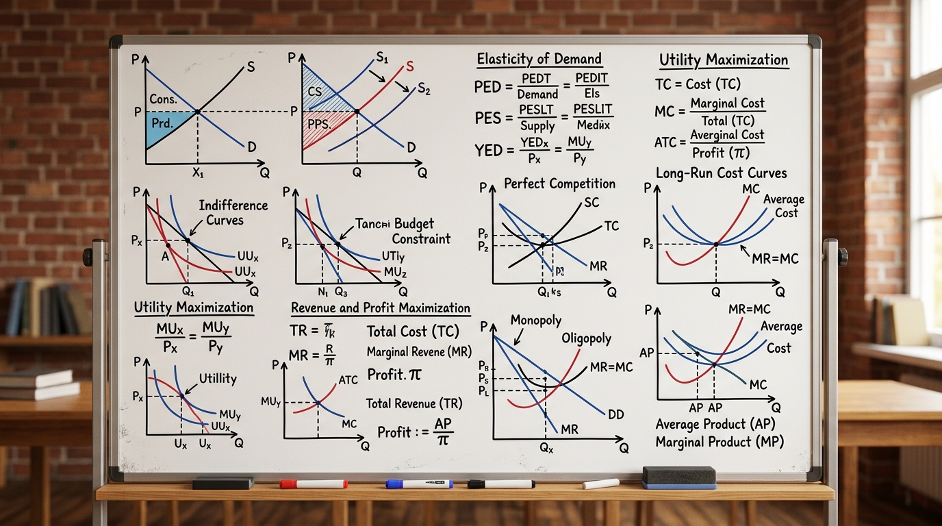
Microeconomics Formula Sheet & Key Theorems: The Complete DU Reference Guide
The ultimate cheat sheet for Intermediate Microeconomics I & II. Master Consumer Theory, Producer Theory, Market Structures, Game Theory, and Welfare Economics.
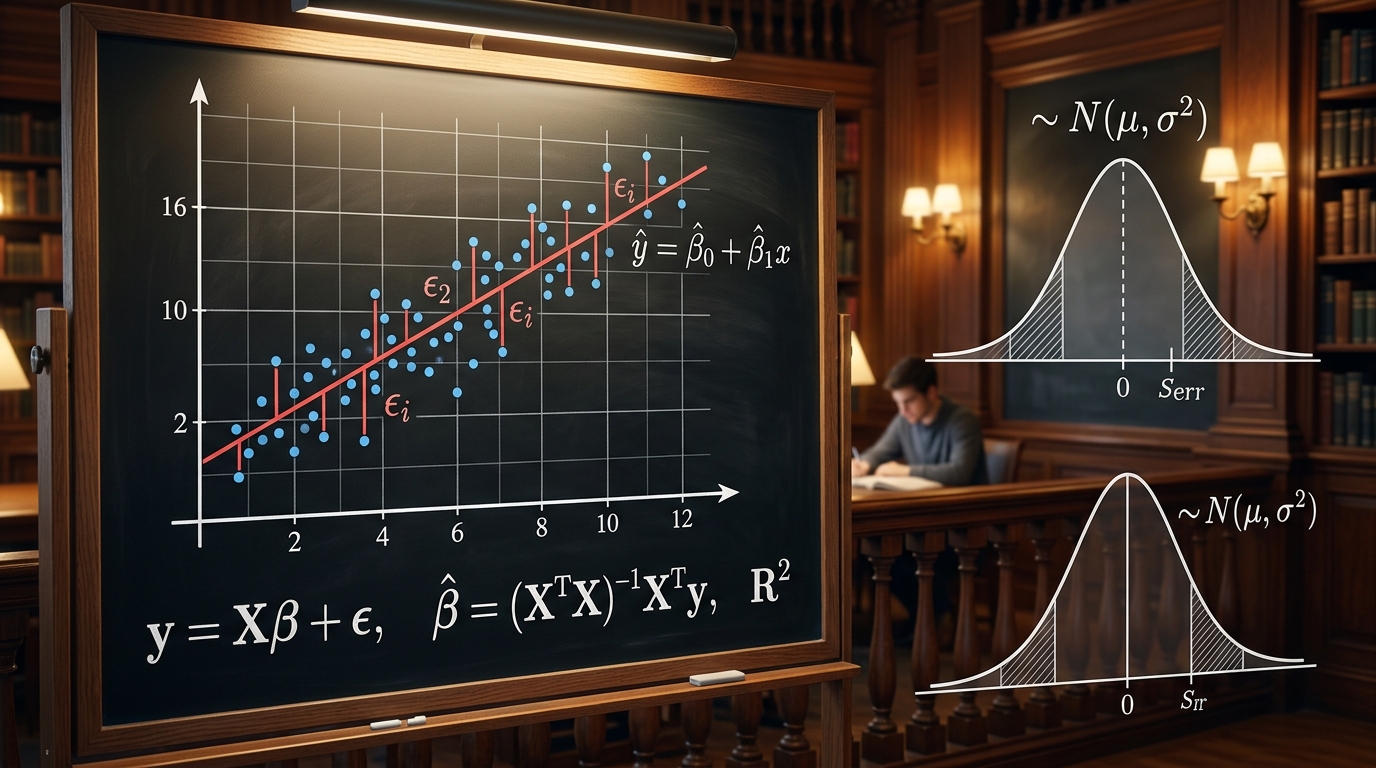
Introductory Econometrics & OLS Regression: Gauss-Markov Theorem, Proofs & Exam Numericals
Comprehensive 4,500-word masterclass on Introductory Econometrics and Ordinary Least Squares (OLS) for DU Economics students. Covers algebraic derivations of beta_0 and beta_1, Gauss-Markov BLUE proofs, R-squared variance decomposition, hypothesis testing (t and F-tests), and 3 fully worked numerical problems.
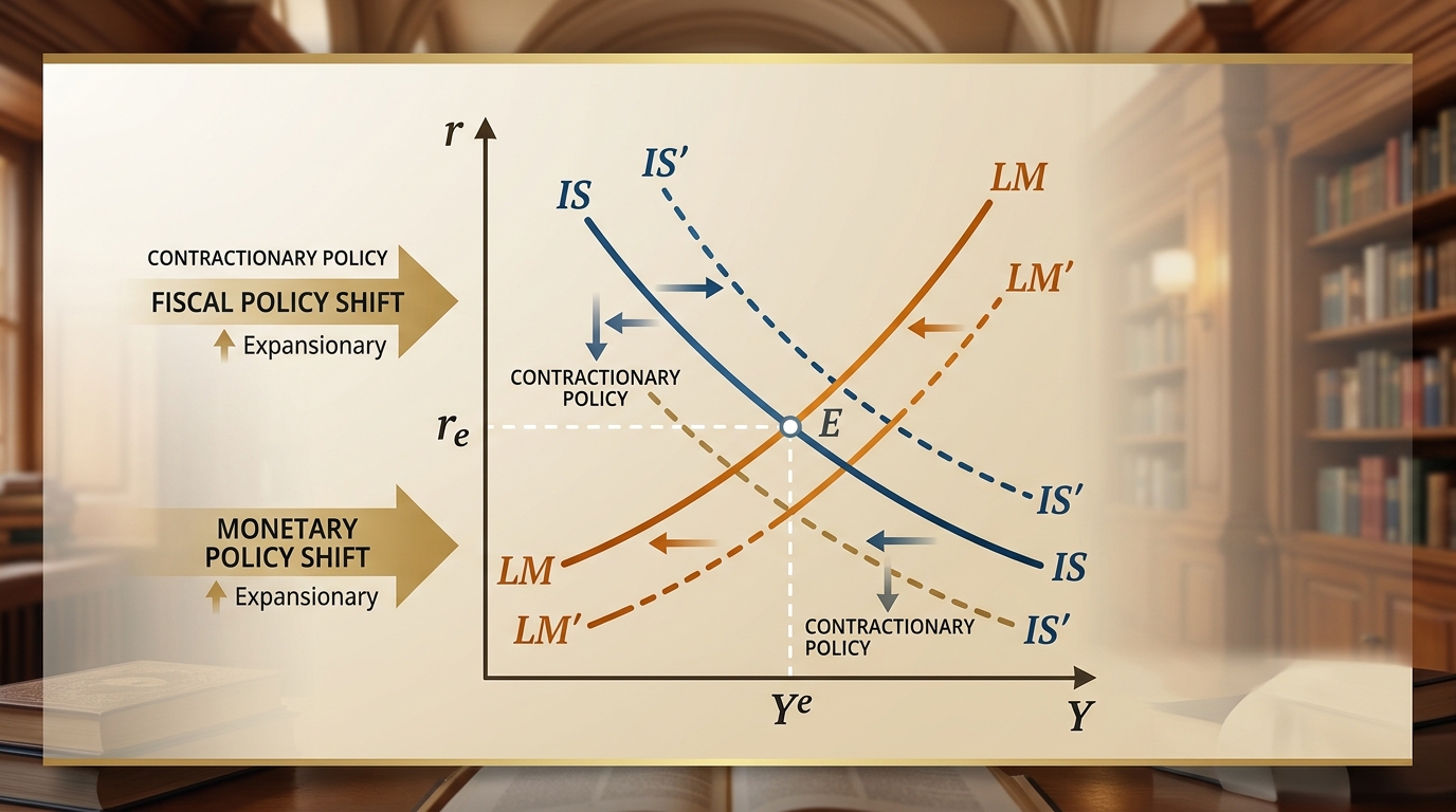
IS-LM Model: Goods & Money Market Equilibrium, Policy Multipliers & DU Exam Numericals
Comprehensive 4,000-word masterclass on the IS-LM model for DU Economics students. Covers algebraic derivations of IS and LM curves, general equilibrium, fiscal and monetary policy multipliers, crowding-out effect, liquidity trap, and 3 fully worked exam numericals.