Introductory Econometrics & OLS Regression: Gauss-Markov Theorem, Proofs & Exam Numericals
Comprehensive 4,500-word masterclass on Introductory Econometrics and Ordinary Least Squares (OLS) for DU Economics students. Covers algebraic derivations of beta_0 and beta_1, Gauss-Markov BLUE proofs, R-squared variance decomposition, hypothesis testing (t and F-tests), and 3 fully worked numerical problems.
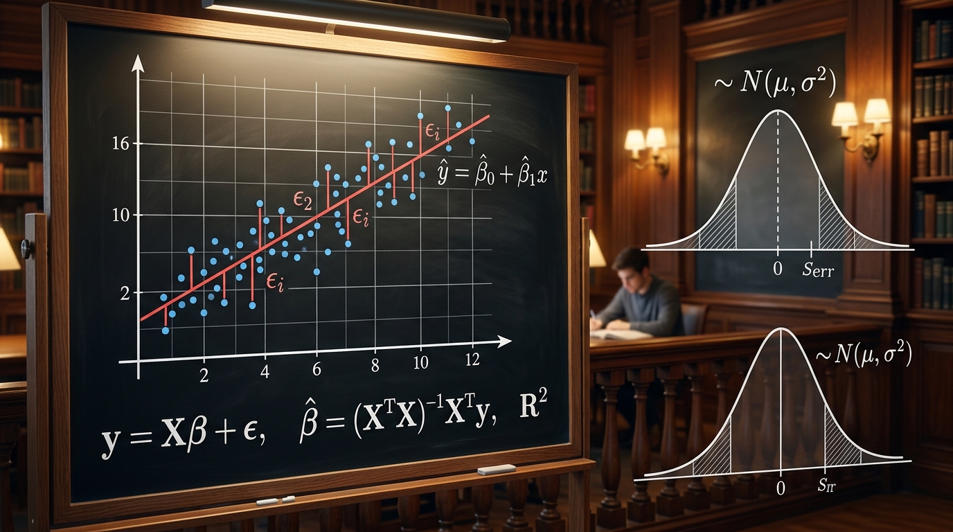
Introductory Econometrics is widely recognized as the most mathematically demanding and conceptually rewarding core course in the Delhi University B.A. (Hons) Economics curriculum (Semester IV Core). It bridges economic theory with empirical data, allowing researchers to quantify relationships, test behavioral hypotheses, and forecast economic phenomena.
At the heart of classical econometrics lies the Ordinary Least Squares (OLS) estimation method. In semester examinations, derivations of OLS estimators, variance proofs under the Classical Linear Regression Model (CLRM), the Gauss-Markov Theorem (BLUE proof), and ANOVA / R-squared variance decompositions constitute over 40% of the question paper.
In this 4,500-word masterclass guide, we derive the simple and multiple OLS estimators from first principles, step through the 7 Classical Linear Regression Model assumptions, prove unbiasedness and minimum variance (Gauss-Markov Theorem), establish hypothesis testing mechanics (t-statistic, p-values, F-tests), and solve 3 complete examination numerical problems.
1. The Simple Linear Regression Model (SLRM) Setup
The Population Regression Function (PRF) describes the stochastic relationship between a dependent variable Y and an explanatory variable X:
- Y_i: Dependent (explained / response) variable.
- X_i: Independent (explanatory / regressor) variable.
- beta_0: Population intercept (value of Y when X = 0).
- beta_1: Population slope parameter (change in E[Y] per unit change in X: dE[Y]/dX = beta_1).
- u_i: Stochastic error term (unobserved factors affecting Y).
1.1 Sample Regression Function (SRF) & Residuals
Because we observe only a sample of size n from the population, we estimate the PRF using the Sample Regression Function:
The sample residual e_i is the difference between the observed value and the fitted value:
2. Mathematical Derivation of OLS Estimators
The Ordinary Least Squares criterion chooses parameter estimates (beta_0_hat, beta_1_hat) that minimize the Residual Sum of Squares (RSS):
2.1 First-Order Conditions (Normal Equations)
Take partial derivatives of S with respect to beta_0_hat and beta_1_hat and set them equal to zero:
Derivative with respect to beta_0_hat:
Sum(Y_i) - n * beta_0_hat - beta_1_hat * Sum(X_i) = 0
Divide by n (using sample means Y_bar = Sum(Y)/n and X_bar = Sum(X)/n):
Derivative with respect to beta_1_hat:
Sum(X_i * Y_i) - beta_0_hat * Sum(X_i) - beta_1_hat * Sum(X_i^2) = 0
Substitute beta_0_hat = Y_bar - beta_1_hat * X_bar into Normal Equation 2:
Sum(X_i * Y_i) - n * X_bar * Y_bar = beta_1_hat * [ Sum(X_i^2) - n * (X_bar)^2 ]
Expressing in lower-case deviation form where x_i = X_i - X_bar and y_i = Y_i - Y_bar:
2.2 Algebraic Properties of OLS Residuals
- Sum of residuals is zero: Sum(e_i) = 0 (and hence the mean of residuals e_bar = 0).
- Residuals are orthogonal to X: Sum(X_i * e_i) = 0.
- Residuals are orthogonal to fitted values: Sum(Y_hat_i * e_i) = 0.
- The regression line passes through the sample means: (X_bar, Y_bar) always lies on the fitted line.
3. Classical Assumptions of the OLS Model (CLRM)
| Assumption | Mathematical Statement | Economic Interpretation |
|---|---|---|
| A1: Linearity in Parameters | Y = beta_0 + beta_1*X + u | The model is linear in coefficients beta, even if X or Y are non-linear (e.g. log(Y) = beta_0 + beta_1*log(X)). |
| A2: Zero Conditional Mean | E[u_i | X_i] = 0 | Exogeneity. The error term contains no systematic information related to X. Violation causes Endogeneity / Omitted Variable Bias. |
| A3: Homoskedasticity | Var(u_i | X_i) = sigma^2 (Constant) | Equal error variance across all observations. Violation is Heteroskedasticity. |
| A4: No Autocorrelation | Cov(u_i, u_j | X) = 0 for i != j | Errors across different observations are uncorrelated. Critical in time-series data. |
| A5: Variation in X | Sum(x_i^2) > 0, not all X_i are identical | X must take at least two distinct values in the sample. In multiple regression: No Perfect Multicollinearity. |
| A6: Normality (for inference) | u_i ~ i.i.d. Normal(0, sigma^2) | Required for exact finite-sample t-tests and F-tests. |
4. The Gauss-Markov Theorem: BLUE Proof
Theorem Statement: Under Assumptions A1 to A5, the OLS estimators beta_0_hat and beta_1_hat are BLUE (Best Linear Unbiased Estimators). That is, among all linear and unbiased estimators, OLS estimators have the minimum sampling variance.
4.1 Proof of Unbiasedness: E[beta_1_hat] = beta_1
Define the weight w_i = x_i / Sum(x_i^2). Notice that:
- Sum(w_i) = Sum(x_i) / Sum(x_i^2) = 0 (since sum of deviations from mean is zero)
- Sum(w_i * X_i) = Sum(w_i * x_i) = Sum(x_i^2) / Sum(x_i^2) = 1
Now write beta_1_hat as a linear combination of Y_i:
= beta_0 * Sum(w_i) + beta_1 * Sum(w_i * X_i) + Sum(w_i * u_i)
= beta_0 * (0) + beta_1 * (1) + Sum(w_i * u_i)
= beta_1 + Sum(w_i * u_i)
Take conditional expectation on X:
Hence, beta_1_hat is strictly Unbiased.
4.2 Variance of OLS Estimator
= sigma^2 * [ Sum(x_i^2) / (Sum(x_i^2))^2 ] = sigma^2 / Sum(x_i^2)
4.3 Proof of Minimum Variance (Efficiency)
Let beta_1_tilde = Sum(c_i * Y_i) be any other linear unbiased estimator of beta_1. Let c_i = w_i + d_i.
For beta_1_tilde to be unbiased, we require Sum(c_i) = 0 and Sum(c_i * X_i) = 1, which implies Sum(d_i) = 0 and Sum(d_i * x_i) = 0.
= sigma^2 * [ Sum(w_i^2) + Sum(d_i^2) + 2 * Sum(w_i * d_i) ]
Note that Sum(w_i * d_i) = [ 1 / Sum(x_i^2) ] * Sum(x_i * d_i) = 0. Therefore:
Because Sum(d_i^2) >= 0, the variance of any competing linear unbiased estimator is strictly greater than or equal to OLS variance. Equality holds if and only if d_i = 0 for all i (i.e., beta_1_tilde = beta_1_hat). Q.E.D. (OLS is BLUE).
5. Goodness of Fit: R-Squared (R^2) & ANOVA
Total variation in Y is partitioned into Explained and Unexplained components:
Sum[ (Y_i - Y_bar)^2 ] = Sum[ (Y_hat_i - Y_bar)^2 ] + Sum(e_i^2)
The Coefficient of Determination (R^2) measures the proportion of total variation in Y explained by the regression line:
In simple bivariate regression, R^2 is exactly equal to the square of Pearson's correlation coefficient: R^2 = r_XY^2.
6. Worked Examination Numerical Problems
Numerical Problem 1: Full Bivariate OLS Estimation (15 Marks)
Question: A study examines the relationship between study hours per week (X) and exam marks out of 100 (Y) for n = 5 students:
Student 1: X = 2, Y = 50
Student 2: X = 4, Y = 60
Student 3: X = 6, Y = 70
Student 4: X = 8, Y = 75
Student 5: X = 10, Y = 95
(a) Compute OLS estimates beta_0_hat and beta_1_hat.
(b) Compute the sample residual variance s^2 and Standard Error of beta_1_hat.
(c) Test H0: beta_1 = 0 vs H1: beta_1 != 0 at the 5% significance level (t_critical for df=3 is 3.182).
(d) Compute R^2.
Solution:
Step 1: Compute Summary Statistics
Sum(X) = 2 + 4 + 6 + 8 + 10 = 30 ==> X_bar = 30/5 = 6
Sum(Y) = 50 + 60 + 70 + 75 + 95 = 350 ==> Y_bar = 350/5 = 70
Sum(X^2) = 4 + 16 + 36 + 64 + 100 = 220
Sum(x_i^2) = Sum(X^2) - n*(X_bar)^2 = 220 - 5*(36) = 220 - 180 = 40
Sum(X*Y) = 2*50 + 4*60 + 6*70 + 8*75 + 10*95 = 100 + 240 + 420 + 600 + 950 = 2,310
Sum(x_i * y_i) = Sum(X*Y) - n*X_bar*Y_bar = 2,310 - 5*(6)*(70) = 2,310 - 2,100 = 210
Part (a): OLS Coefficients
beta_0_hat = Y_bar - beta_1_hat * X_bar = 70 - 5.25 * 6 = 70 - 31.50 = 38.50
Fitted Line: Y_hat = 38.50 + 5.25 * X
Part (b): Residuals, Variance s^2, and SE(beta_1_hat)
Residuals e_i = Y - Y_hat: +1.0, +0.5, 0.0, -5.5, +4.0
Sum(e_i^2) = 1.0^2 + 0.5^2 + 0.0^2 + (-5.5)^2 + 4.0^2 = 1.0 + 0.25 + 0 + 30.25 + 16.0 = 47.50
Unbiased error variance s^2 = RSS / (n - 2) = 47.50 / (5 - 2) = 47.50 / 3 = 15.833
s = sqrt(15.833) = 3.979
SE(beta_1_hat) = sqrt[ s^2 / Sum(x_i^2) ] = sqrt[ 15.833 / 40 ] = sqrt(0.3958) = 0.629
Part (c): Hypothesis Testing (t-test)
Since |t_calc| = 8.35 > t_crit (3.182), we REJECT the null hypothesis H0 at the 5% level.
Conclusion: Study hours have a statistically significant positive effect on exam marks.
Part (d): Coefficient of Determination R^2
TSS = Sum(Y^2) - n*(Y_bar)^2 = 25,650 - 5*(4,900) = 25,650 - 24,500 = 1,150
ESS = TSS - RSS = 1,150 - 47.50 = 1,102.50
R^2 = ESS / TSS = 1,102.50 / 1,150 = 0.9587 (or 95.87%)
Numerical Problem 2: ANOVA Table & F-Test (10 Marks)
Question: For a regression with n = 22 observations and k = 3 explanatory variables (X1, X2, X3), total sum of squares TSS = 500 and residual sum of squares RSS = 100.
(a) Construct the ANOVA Table.
(b) Test the overall significance of the regression at the 1% level (F_critical for df=(3, 18) is 5.09).
Solution:
| Source of Variation | Sum of Squares (SS) | Degrees of Freedom (df) | Mean Square (MS) | F-Statistic |
|---|---|---|---|---|
| Regression (ESS) | 400 (500 - 100) | k = 3 | 400 / 3 = 133.33 | F = 133.33 / 5.56 = 24.00 |
| Residual (RSS) | 100 | n - k - 1 = 22 - 3 - 1 = 18 | 100 / 18 = 5.56 | |
| Total (TSS) | 500 | n - 1 = 21 | - | - |
Conclusion: Since F_calculated = 24.00 > F_critical = 5.09, we reject H0: beta_1 = beta_2 = beta_3 = 0. The regression model is jointly highly significant at the 1% level.
7. Summary Checklist for Econometrics Exams
- State all 5 Gauss-Markov assumptions clearly before writing proofs.
- Remember the derivation shorthand: beta_1_hat = Sum(w_i * Y_i) where w_i = x_i / Sum(x_i^2).
- Degrees of freedom for residual variance in SLRM is always n - 2. In multiple regression with k slopes, df = n - k - 1.
- R^2 increases monotonically whenever a new variable is added, which is why Adjusted R^2 is preferred for model comparison.
For related mathematical economics guides, see our MME Distinction Masterclass and Cobb-Douglas Mathematical Proofs.
Frequently asked questions
What does BLUE stand for in the Gauss-Markov Theorem?
BLUE stands for Best Linear Unbiased Estimator. 'Best' means having the minimum sampling variance among all linear, unbiased estimators.
Why is the degrees of freedom for residual variance (n - 2) in simple linear regression?
Because two degrees of freedom are lost in estimating the two sample parameters: intercept beta_0 and slope beta_1.
Dhairya sat the same DU papers he now writes about. Acadly is his attempt to say the useful things his own first-year self would have wanted to hear.
Keep reading
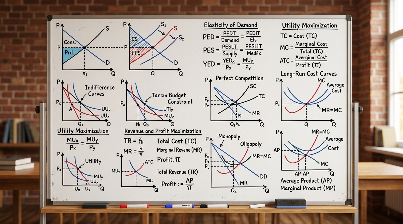
Microeconomics Formula Sheet & Key Theorems: The Complete DU Reference Guide
The ultimate cheat sheet for Intermediate Microeconomics I & II. Master Consumer Theory, Producer Theory, Market Structures, Game Theory, and Welfare Economics.
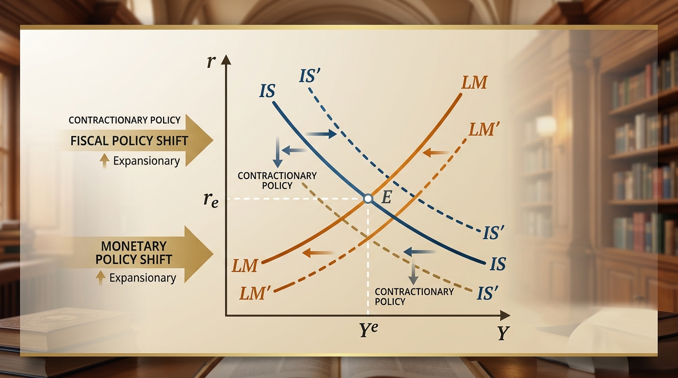
IS-LM Model: Goods & Money Market Equilibrium, Policy Multipliers & DU Exam Numericals
Comprehensive 4,000-word masterclass on the IS-LM model for DU Economics students. Covers algebraic derivations of IS and LM curves, general equilibrium, fiscal and monetary policy multipliers, crowding-out effect, liquidity trap, and 3 fully worked exam numericals.

Oligopoly Models: Cournot, Bertrand & Stackelberg — Complete Derivations & DU Exam Numericals
Comprehensive 4,000-word masterclass on Oligopoly Models for DU Economics students. Covers Cournot quantity competition, Bertrand price competition, Stackelberg leader-follower equilibrium, and 3 step-by-step worked numerical problems.