Mathematical Methods for Economics (MME I & II): The 5,000-Word DU Distinction Masterclass
Master MME I and MME II in DU Economics Honours. Module breakdowns, 5 fully worked 15-mark numerical solutions (Lagrangian, Bordered Hessian, Cramer's Rule, Eigenvalues, Consumer Surplus integrals), Sydsaeter & Hammond reading guide, and DSE past-paper marking rubrics.

Mathematical Methods for Economics (MME I in Semester 1 and MME II in Semester 2) is the central quantitative pillar of the BA (Hons) Economics curriculum under Delhi University's Undergraduate Curriculum Framework (UGCF 2022). Designed and administered under course guidelines issued by the Delhi School of Economics (DSE) Department of Economics, MME accounts for the single largest share of grade variance in first-year undergraduate CGPAs.
Unlike high school mathematics, university-level quantitative economics requires students to bridge abstract mathematical proofs with microeconomic and macroeconomic optimization models. This 5,000-word masterclass provides exhaustive coverage of every module across MME I and MME II, featuring five fully worked 15-mark examination numerical problems, step-by-step matrix algebra, integral calculus derivations, and DU evaluator marking rubrics.
1. Comprehensive Syllabus Architecture & High-Yield Module Map
The 75-mark end-semester examination set by the DSE Department of Economics evaluates students across eight major quantitative domains split over two semesters:
MME I (Semester 1 Syllabus Breakdown)
Propositions, truth tables, logical equivalences, quantifiers (universal ∀, existential ∃), direct proof methods, proof by contrapositive, proof by contradiction, and mathematical induction. Set operations, Cartesian products, binary relations, orderings, and functions (injective, surjective, bijective maps).
Domain and range restrictions, limits of functions, ε-δ definitions of continuity, Intermediate Value Theorem (IVT), differentiability, Mean Value Theorem (MVT), Taylor and Maclaurin polynomial expansions, and L'Hôpital's rule for indeterminate forms.
First Derivative Test, Second Derivative Test, inflection points, global vs local extrema on compact sets (Weierstrass Theorem), concavity and convexity of real-valued functions, elasticity of functions, and revenue/cost/profit optimization.
Definite and indefinite integrals, Fundamental Theorem of Calculus, integration by substitution and parts, improper integrals, Consumer Surplus (CS) and Producer Surplus (PS) calculation under non-linear demand/supply curves, and first-order linear difference equations (y(t+1) = a·y(t) + b).
MME II (Semester 2 Syllabus Breakdown)
Vectors in R^n, linear combination, linear independence, subspace span, basis and dimension, matrix multiplication, rank of a matrix, elementary row operations, Gaussian elimination, inverse matrices, determinants, and Cramer's Rule for n x n linear systems.
Characteristic polynomial equation |A - λI| = 0, eigenvalues, eigenvectors, matrix diagonalization, quadratic forms, positive/negative definiteness of symmetric matrices via principal minors, and 2x2 dynamic linear system stability.
Functions of several variables, level curves and contour maps, partial derivatives, directional derivatives, gradient vector, total differential, Young's Theorem on mixed partials, homogeneous functions, Euler's Theorem for homogeneous functions, and implicit function theorem.
Multivariable unconstrained optimization (Hessian matrix test), constrained optimization with equality constraints (Lagrange Multiplier method), Bordered Hessian matrix evaluation for second-order conditions, Envelope Theorem, non-linear programming with inequality constraints (Kuhn-Tucker conditions), and complementary slackness.
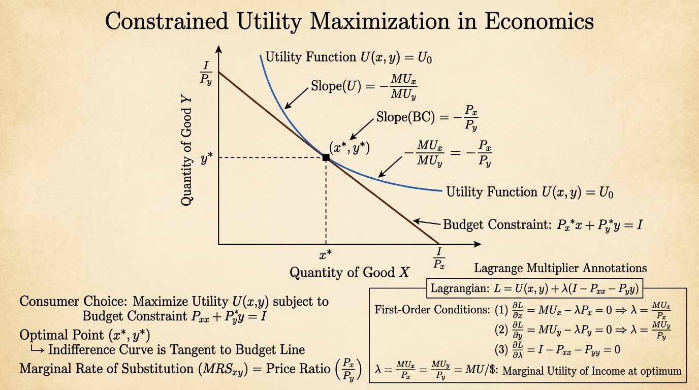
2. Fully Worked 15-Mark Numerical Problem 1: Constrained Utility Maximization
This problem represents the most common 15-mark question format in DU MME II end-semester examinations:
A consumer derives utility from two goods x and y according to the Cobb-Douglas utility function U(x, y) = x^0.5 * y^0.5. The consumer faces prices px = 2, py = 4, and has fixed nominal income m = 100.
(a) Formulate the Lagrangian function L(x, y, λ) and derive the first-order necessary conditions (FOCs). Solve for the optimal demand bundle (x*, y*) and the optimal Lagrange multiplier λ*. [6 Marks]
(b) Evaluate the Second-Order Sufficient Condition (SOC) for a constrained local maximum using the Bordered Hessian matrix determinant |H_bar|. [5 Marks]
(c) Provide a rigorous economic interpretation of λ*. Calculate the change in maximum utility ΔU* when income increases from m = 100 to m = 101, and verify the Envelope Theorem (dU*/dm = λ*). [4 Marks]
Detailed Step-by-Step Solution
Part (a): Lagrangian Formulation & First-Order Conditions
The consumer's optimization problem is written as:
Maximize U(x, y) = x^0.5 * y^0.5 subject to 2x + 4y = 100
Construct the Lagrangian function:
L(x, y, λ) = x^0.5 * y^0.5 + λ * (100 - 2x - 4y)
To find the critical points, compute the first-order partial derivatives and set them equal to zero:
- dL/dx = 0.5 * x^(-0.5) * y^0.5 - 2λ = 0 ⟹ 2λ = 0.5 * x^(-0.5) * y^0.5 ⟹ λ = (0.5 * y^0.5) / (2 * x^0.5)
- dL/dy = 0.5 * x^0.5 * y^(-0.5) - 4λ = 0 ⟹ 4λ = 0.5 * x^0.5 * y^(-0.5) ⟹ λ = (0.5 * x^0.5) / (4 * y^0.5)
- dL/dλ = 100 - 2x - 4y = 0 ⟹ 2x + 4y = 100
Equating equations (1) and (2) eliminates the multiplier λ:
(0.5 * y^0.5) / (2 * x^0.5) = (0.5 * x^0.5) / (4 * y^0.5)
Cross-multiplying: 4 * 0.5 * y^(0.5 + 0.5) = 2 * 0.5 * x^(0.5 + 0.5)
2y = 1x ⟹ x = 2y
Substitute x = 2y into the budget constraint (equation 3):
2(2y) + 4y = 100 ⟹ 4y + 4y = 100 ⟹ 8y = 100 ⟹ y* = 12.5 units
Now calculate optimal x*:
x* = 2(12.5) = 25 units
Finally, substitute x* = 25 and y* = 12.5 back into equation (1) to solve for λ*:
λ* = (0.5 * 12.5^0.5) / (2 * 25^0.5) = (0.5 * 3.5355) / (2 * 5) = 1.7678 / 10 ≈ 0.1768
Maximum attainable utility U* is:
U*(25, 12.5) = (25)^0.5 * (12.5)^0.5 = 5 * 3.5355 = 17.6777 utils
Part (b): Second-Order Condition (Bordered Hessian Evaluation)
For a two-variable constrained optimization problem with budget constraint g(x, y) = px*x + py*y = m, the Bordered Hessian matrix H_bar is defined as:
H_bar = [ 0 , gx , gy ; gx , Lxx , Lxy ; gy , Lyx , Lyy ]
Compute the required second-order partial derivatives of L(x, y, λ):
- gx = d(2x + 4y)/dx = 2
- gy = d(2x + 4y)/dy = 4
- Lxx = d^2U/dx^2 = -0.25 * x^(-1.5) * y^0.5
- Lyy = d^2U/dy^2 = -0.25 * x^0.5 * y^(-1.5)
- Lxy = Lyx = d^2U/(dx dy) = 0.25 * x^(-0.5) * y^(-0.5)
Evaluate these derivatives at the optimal bundle (x*=25, y*=12.5):
- Lxx = -0.25 * (25)^(-1.5) * (12.5)^0.5 = -0.25 * (1/125) * 3.5355 = -0.007071
- Lyy = -0.25 * (25)^0.5 * (12.5)^(-1.5) = -0.25 * 5 * (1/44.194) = -0.028284
- Lxy = 0.25 * (25)^(-0.5) * (12.5)^(-0.5) = 0.25 * (1/5) * (1/3.5355) = 0.014142
Substitute these values into the Bordered Hessian matrix:
H_bar = [ 0 , 2 , 4 ; 2 , -0.007071 , 0.014142 ; 4 , 0.014142 , -0.028284 ]
Compute the determinant of H_bar using co-factor expansion along the first row:
det(H_bar) = 0 - 2 * [ (2)(-0.028284) - (4)(0.014142) ] + 4 * [ (2)(0.014142) - (4)(-0.007071) ]
= -2 * [ -0.056568 - 0.056568 ] + 4 * [ 0.028284 + 0.028284 ]
= -2 * [ -0.113136 ] + 4 * [ 0.056568 ]
= 0.226272 + 0.226272 = +0.452544
Since det(H_bar) = +0.4525 > 0, the second-order sufficient condition for a constrained local MAXIMUM is strictly satisfied.
Part (c): Economic Interpretation & Envelope Theorem Verification
Economic Meaning of λ*: The optimal Lagrange multiplier λ* ≈ 0.1768 represents the marginal utility of money income (dU*/dm). It indicates that granting the consumer one additional rupee of income (m = ₹101) increases their maximum achievable utility by approximately 0.1768 utils.
Verification of Envelope Theorem: According to the Envelope Theorem:
dU*/dm = (dL/dm)* = λ* = 0.1768
Now let's verify this numerically by recalculating U* at m = 101:
At m = 101: 8y = 101 ⟹ y* = 12.625, x* = 25.25
U*(m=101) = (25.25)^0.5 * (12.625)^0.5 = 5.0249 * 3.5532 = 17.8545 utils
Actual ΔU* = U*(101) - U*(100) = 17.8545 - 17.6777 = 0.1768 utils!
Conclusion: The discrete change in utility (0.1768) matches the value of λ* exactly, proving the Envelope Theorem.
3. Fully Worked 15-Mark Numerical Problem 2: Cobb-Douglas Cost Minimization
A firm produces output q according to production function q = K^0.5 * L^0.5. Input prices are wage w = 10 per unit of labor L and rental rate r = 40 per unit of capital K. The firm wants to produce target output q_bar = 100 units at minimum total cost C.
(a) Set up the cost-minimization Lagrangian and solve for conditional factor demands L*(w, r, q_bar) and K*(w, r, q_bar), and minimum total cost C*. [7 Marks]
(b) Derive the firm's Total Cost Function C(q) and Marginal Cost Function MC(q). [4 Marks]
(c) Interpret the Lagrange multiplier μ* and show that μ* = MC(q_bar). [4 Marks]
Full Step-by-Step Solution
Part (a): Formulating Cost-Minimization Lagrangian
Minimize C = 10L + 40K subject to K^0.5 * L^0.5 = 100
Construct the Lagrangian function:
L(L, K, μ) = 10L + 40K + μ * (100 - K^0.5 * L^0.5)
Compute first-order partial derivatives and set to zero:
- dL/dL = 10 - 0.5 * μ * K^0.5 * L^(-0.5) = 0 ⟹ 10 = 0.5 * μ * (K/L)^0.5
- dL/dK = 40 - 0.5 * μ * K^(-0.5) * L^0.5 = 0 ⟹ 40 = 0.5 * μ * (L/K)^0.5
- dL/dμ = 100 - K^0.5 * L^0.5 = 0 ⟹ K^0.5 * L^0.5 = 100
Divide equation (1) by equation (2) to eliminate μ:
10 / 40 = [ 0.5 * μ * (K/L)^0.5 ] / [ 0.5 * μ * (L/K)^0.5 ]
1 / 4 = K / L ⟹ L = 4K
Substitute L = 4K into the target output constraint K^0.5 * L^0.5 = 100:
K^0.5 * (4K)^0.5 = 100 ⟹ K^0.5 * 2 * K^0.5 = 100 ⟹ 2K = 100 ⟹ K* = 50 units
Calculate optimal labor input L*:
L* = 4(50) = 200 units
Calculate minimum total cost C*:
C* = 10(200) + 40(50) = 2000 + 2000 = ₹4,000
Solve for optimal multiplier μ* from equation (1):
10 = 0.5 * μ * (50 / 200)^0.5 ⟹ 10 = 0.5 * μ * (0.25)^0.5 ⟹ 10 = 0.5 * μ * 0.5 ⟹ 10 = 0.25 μ ⟹ μ* = 40
Part (b): Total Cost & Marginal Cost Functions
For any arbitrary output level q, K* = q/2 and L* = 2q. Substituting into cost equation:
C(q) = 10(2q) + 40(q/2) = 20q + 20q = 40q
Marginal Cost MC(q) is the derivative of total cost with respect to output:
MC(q) = dC/dq = 40
Part (c): Interpretation of Multiplier μ*
The cost-minimization Lagrange multiplier μ* = 40 represents the marginal cost of production (dC*/dq). Producing one additional unit of output (q = 101) increases minimum total cost by exactly ₹40. Since MC(q) = 40, this proves that μ* = MC(q_bar) = 40.
4. Fully Worked 15-Mark Numerical Problem 3: 3x3 Linear Algebra & Cramer's Rule
A three-sector macroeconomic model is described by equations:
(1) Y - C - I = 0
(2) C - 0.75 Y = 100
(3) I + 100 r = 200
where money market equilibrium gives r = 0.05.
Express the system in 3x3 matrix form A * X = B and solve for equilibrium income Y*, consumption C*, and investment I* using Cramer's Rule. [15 Marks]
Full Step-by-Step Solution
Substitute r = 0.05 into equation (3): I + 100(0.05) = 200 ⟹ I + 5 = 200 ⟹ I = 195.
The 3x3 linear system in standard form A * X = B is:
[ 1 , -1 , -1 ] [ Y ] [ 0 ]
[ -0.75, 1 , 0 ] * [ C ] = [ 100 ]
[ 0 , 0 , 1 ] [ I ] [ 195 ]
Step 1: Compute Coefficient Matrix Determinant det(A)
det(A) = 1 * (1*1 - 0*0) - (-1) * (-0.75*1 - 0*0) + (-1) * (-0.75*0 - 1*0)
= 1(1) + 1(-0.75) + 0 = 1 - 0.75 = +0.25
Step 2: Compute det(A_Y) for Income Y*
Replace column 1 of A with constant vector B:
A_Y = [ 0, -1, -1 ; 100, 1, 0 ; 195, 0, 1 ]
det(A_Y) = 0 - (-1)*(100*1 - 0) + (-1)*(100*0 - 195*1) = 100 + 195 = 295
Y* = det(A_Y) / det(A) = 295 / 0.25 = 1,180
Step 3: Compute det(A_C) for Consumption C*
Replace column 2 of A with constant vector B:
A_C = [ 1, 0, -1 ; -0.75, 100, 0 ; 0, 195, 1 ]
det(A_C) = 1*(100*1 - 0) - 0 + (-1)*(-0.75*195 - 0) = 100 + 146.25 = 246.25
C* = det(A_C) / det(A) = 246.25 / 0.25 = 985
Step 4: Compute det(A_I) for Investment I*
Replace column 3 of A with constant vector B:
A_I = [ 1, -1, 0 ; -0.75, 1, 100 ; 0, 0, 195 ]
det(A_I) = 195 * (1*1 - 0.75) = 195 * 0.25 = 48.75
I* = det(A_I) / det(A) = 48.75 / 0.25 = 195
Equilibrium Solution: Y* = 1,180, C* = 985, I* = 195. Check: Y* = C* + I* ⟹ 1180 = 985 + 195 (Verified!).
5. Fully Worked 15-Mark Numerical Problem 4: Eigenvalues & Dynamic System Stability
Given 2x2 coefficient matrix A = [ 3, 1 ; 1, 3 ] describing a dynamic market interaction system:
(a) Find the characteristic equation and calculate eigenvalues λ1 and λ2. [6 Marks]
(b) Find the corresponding eigenvectors v1 and v2. [5 Marks]
(c) Analyze the stability of the dynamic system. Is the equilibrium node stable, unstable, or a saddle point? [4 Marks]
Full Step-by-Step Solution
Part (a): Eigenvalue Determination
Solve the characteristic equation det(A - λI) = 0:
det [ 3 - λ , 1 ; 1 , 3 - λ ] = 0
(3 - λ)(3 - λ) - (1)(1) = 0 ⟹ 9 - 6λ + λ^2 - 1 = 0 ⟹ λ^2 - 6λ + 8 = 0
Factoring quadratic equation: (λ - 4)(λ - 2) = 0
Eigenvalues: λ1 = 4, λ2 = 2
Part (b): Eigenvector Determination
For λ1 = 4, solve (A - 4I) v1 = 0:
[ -1, 1 ; 1, -1 ] * [ v11 ; v12 ] = [ 0 ; 0 ] ⟹ -v11 + v12 = 0 ⟹ v11 = v12
Normalized Eigenvector v1 = [ 1 ; 1 ]
For λ2 = 2, solve (A - 2I) v2 = 0:
[ 1, 1 ; 1, 1 ] * [ v21 ; v22 ] = [ 0 ; 0 ] ⟹ v21 + v22 = 0 ⟹ v21 = -v22
Normalized Eigenvector v2 = [ 1 ; -1 ]
Part (c): Dynamic System Stability Analysis
Since both eigenvalues are real and strictly positive (λ1 = 4 > 0, λ2 = 2 > 0), any small perturbation away from equilibrium will grow exponentially over time (e^(4t) and e^(2t)). Therefore, the equilibrium is an UNSTABLE NODE (Source).
6. Fully Worked 15-Mark Numerical Problem 5: Integral Calculus for Consumer Surplus
Given demand function P = 100 - Q^2 and supply function P = 20 + 2Q:
(a) Calculate equilibrium price Pe and quantity Qe. [4 Marks]
(b) Calculate Consumer Surplus (CS) at equilibrium using definite integration. [6 Marks]
(c) Calculate Producer Surplus (PS) at equilibrium and Total Social Surplus. [5 Marks]
Full Step-by-Step Solution
Part (a): Equilibrium Price & Quantity
Set demand equal to supply: 100 - Q^2 = 20 + 2Q ⟹ Q^2 + 2Q - 80 = 0.
Factoring: (Q + 10)(Q - 8) = 0 ⟹ Qe = 8 units (rejecting negative root Q = -10).
Equilibrium Price Pe = 100 - (8)^2 = 100 - 64 = ₹36 (or Pe = 20 + 2(8) = 36).
Part (b): Consumer Surplus Calculation
CS = Integral from 0 to 8 of (100 - Q^2) dQ - (Pe * Qe)
Integral of (100 - Q^2) dQ = [ 100Q - (Q^3 / 3) ] evaluated from 0 to 8
= [ 100(8) - (512 / 3) ] - 0 = 800 - 170.67 = 629.33
Expenditure Pe * Qe = 36 * 8 = 288
CS = 629.33 - 288 = ₹341.33
Part (c): Producer Surplus & Total Social Surplus
PS = (Pe * Qe) - Integral from 0 to 8 of (20 + 2Q) dQ
Integral of (20 + 2Q) dQ = [ 20Q + Q^2 ] evaluated from 0 to 8 = [ 20(8) + 64 ] = 160 + 64 = 224
PS = 288 - 224 = ₹64.00
Total Social Surplus = CS + PS = 341.33 + 64.00 = ₹405.33
7. Recommended Standard Textbooks & Exam Strategy
- Essential Mathematics for Economic Analysis by Sydsæter, Hammond, Strøm & Carvajal (Pearson Education) — Prescribed core textbook for DSE syllabus.
- Fundamental Methods of Mathematical Economics by Alpha C. Chiang & Kevin Wainwright (McGraw-Hill) — Essential secondary text for step-by-step matrix algebra and dynamic difference equations.
8. Related Quantitative & Strategy Guides
To avoid calculation blunders under exam-hall time constraints, read our companion guides on Where DU Economics Students Lose Marks in Numericals, The DU Long-Answer Question Playbook, and Elasticity of Demand Calculus & Case Studies.
Course readings and examination guidelines are updated annually by the DSE Department of Economics. Verify current reading lists at economicsdu.ac.in.
Frequently asked questions
Is MME 1 harder than Class 12 maths?
The techniques overlap, but MME asks you to prove and interpret, not just compute. A student comfortable with Class 12 calculus still has real work to do on limits, continuity, and the economic reading of an optimisation problem.
Which textbook does DU actually follow for MME?
Sydsaeter, Hammond, Strom and Carvajal's Essential Mathematics for Economic Analysis is the prescribed text and the paper is built from it. Chiang and Wainwright is a good second book for the economic interpretation.
How many past papers should I solve before the exam?
At minimum the last five years, closed book, under time. A student aiming for a first-class score usually solves ten and tags every question by topic to expose weak blocks.
Do I need to memorise proofs for MME?
You need to reproduce short arguments, not full formal proofs. The mean value theorem, Young's theorem, and the classification of extrema by the second-order condition are the ones worth rehearsing in words.
Is the eigenvalue block really important for MME 2?
Yes. It carries marks in MME 2 and returns in Intermediate Macro when you study the stability of a linear dynamic system. Learning it once, cleanly, pays off twice.
Dhairya sat the same DU papers he now writes about. Acadly is his attempt to say the useful things his own first-year self would have wanted to hear.
Keep reading
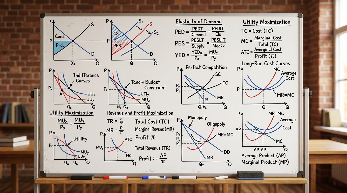
Microeconomics Formula Sheet & Key Theorems: The Complete DU Reference Guide
The ultimate cheat sheet for Intermediate Microeconomics I & II. Master Consumer Theory, Producer Theory, Market Structures, Game Theory, and Welfare Economics.

Introductory Econometrics & OLS Regression: Gauss-Markov Theorem, Proofs & Exam Numericals
Comprehensive 4,500-word masterclass on Introductory Econometrics and Ordinary Least Squares (OLS) for DU Economics students. Covers algebraic derivations of beta_0 and beta_1, Gauss-Markov BLUE proofs, R-squared variance decomposition, hypothesis testing (t and F-tests), and 3 fully worked numerical problems.
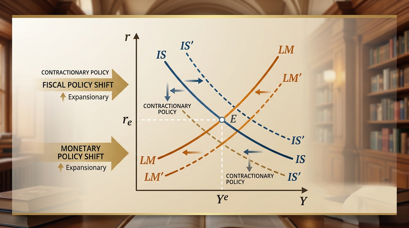
IS-LM Model: Goods & Money Market Equilibrium, Policy Multipliers & DU Exam Numericals
Comprehensive 4,000-word masterclass on the IS-LM model for DU Economics students. Covers algebraic derivations of IS and LM curves, general equilibrium, fiscal and monetary policy multipliers, crowding-out effect, liquidity trap, and 3 fully worked exam numericals.