IS-LM Model: Goods & Money Market Equilibrium, Policy Multipliers & DU Exam Numericals
Comprehensive 4,000-word masterclass on the IS-LM model for DU Economics students. Covers algebraic derivations of IS and LM curves, general equilibrium, fiscal and monetary policy multipliers, crowding-out effect, liquidity trap, and 3 fully worked exam numericals.
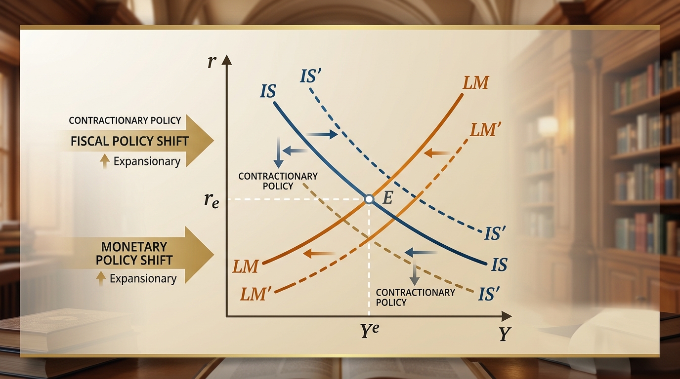
The IS-LM Model (Investment-Savings / Liquidity Preference-Money Supply), developed by Sir John Hicks in 1937 and expanded by Alvin Hansen, is the cornerstone of short-run macroeconomic analysis. It integrates the goods market (real sector) and the money market (financial sector) to determine simultaneous general equilibrium values for national income (Y) and the interest rate (r).
For undergraduate students in Delhi University's B.A. (Hons) Economics and B.A. Programme (Intermediate Macroeconomics I & II), the IS-LM model represents a compulsory 15-mark to 20-mark analytical and numerical block in semester examinations.
In this 4,000-word masterclass guide, we derive the algebraic equations of the IS and LM curves, calculate general equilibrium (Y*, r*), derive government expenditure and money supply multipliers, analyze the crowding-out effect and extreme cases (liquidity trap, classical case), and solve 3 step-by-step examination numerical problems.
1. The Goods Market Equilibrium (The IS Curve)
The IS curve represents all combinations of interest rates (r) and national income levels (Y) at which the goods market is in equilibrium, i.e., aggregate demand equals national income (Y = AD), or planned investment equals planned savings (I = S).
1.1 Component Equations of Goods Market
- Consumption Function: C = C_bar + c * (Y - T), where C_bar > 0 is autonomous consumption, c is Marginal Propensity to Consume (0 < c < 1), and T is lump-sum taxes.
- Investment Function: I = I_bar - d * r, where I_bar is autonomous investment and d > 0 measures investment sensitivity to interest rates.
- Government Spending: G = G_bar (exogenous).
- Net Exports (Closed Economy): NX = 0.
1.2 Algebraic Derivation of the IS Curve
Goods market equilibrium condition:
Y = C_bar + c*(Y - T) + I_bar - d*r + G_bar
Group all terms containing Y on the left-hand side:
(1 - c)*Y = A_bar - d*r
where A_bar = C_bar - c*T + I_bar + G_bar is total autonomous spending.
Solving for Y as a function of r yields the IS Curve Equation:
where alpha_G = 1 / (1 - c) is the simple Keynesian autonomous expenditure multiplier.
Alternatively, solving for r as a function of Y (Inverse IS Curve):
1.3 Slope and Position of the IS Curve
- Slope of IS Curve: - (1 - c) / d. The IS curve is downward sloping because a higher interest rate increases borrowing costs, reduces investment demand, and via the multiplier process lowers equilibrium income Y.
- Steepness: The IS curve is steeper if d is small (investment is insensitive to interest rate) or if MPC c is small (multiplier is small).
- Shifts: An increase in autonomous spending (G_bar, C_bar, I_bar) or a decrease in taxes (T) shifts the IS curve to the right by delta_G * alpha_G.
2. The Money Market Equilibrium (The LM Curve)
The LM curve represents all combinations of interest rates (r) and income levels (Y) at which money demand equals real money supply (L = M/P).
2.1 Demand and Supply of Real Money Balances
- Real Money Supply: M_bar / P (exogenous, fixed by central bank).
- Real Money Demand (Keynesian Liquidity Preference): L(Y, r) = k * Y - h * r, where k > 0 measures transaction demand sensitivity to income, and h > 0 measures speculative demand sensitivity to interest rates.
2.2 Algebraic Derivation of the LM Curve
Money market equilibrium condition:
Solving for r yields the Inverse LM Curve Equation:
Solving for Y as a function of r:
2.3 Slope and Position of the LM Curve
- Slope of LM Curve: k / h. The LM curve is upward sloping because higher income Y increases transaction money demand; to restore money market equilibrium with a fixed money supply, the interest rate r must rise to reduce speculative money demand.
- Steepness: The LM curve is steeper if k is large or if h is small (money demand is insensitive to interest rate).
- Shifts: An increase in real money supply (M_bar / P) shifts the LM curve to the right by (1 / k) * delta(M/P).
3. Simultaneous General Equilibrium (Y*, r*)
General equilibrium occurs at the intersection of the IS and LM curves, where both the goods market and money market clear simultaneously.
LM: r = (k / h) * Y - (1 / h) * (M/P)
Substitute r from LM into IS:
Y + alpha_G * d * (k / h) * Y = alpha_G * A_bar + (alpha_G * d / h) * (M/P)
Y * [ 1 + alpha_G * d * k / h ] = alpha_G * A_bar + (alpha_G * d / h) * (M/P)
Solving for Equilibrium Income Y*:
where gamma = alpha_G / [ 1 + alpha_G * d * k / h ] = h * alpha_G / (h + d * k * alpha_G) is the Fiscal Policy Multiplier in the IS-LM framework.
Note that since gamma < alpha_G, fiscal policy is LESS effective in IS-LM than in the simple Keynesian multiplier framework due to the crowding-out effect.
4. Fiscal and Monetary Policy Effectiveness
| Case / Extreme Scenario | LM Curve Shape | Fiscal Policy (dG) | Monetary Policy (dM) |
|---|---|---|---|
| Liquidity Trap (h -> infinity) | Horizontal (r = r_min) | Maximal (Full Keynesian multiplier, 0 crowding out) | Completely Ineffective (dY = 0) |
| Classical Case (h -> 0) | Vertical (Y = (1/k)*M/P) | Completely Ineffective (100% crowding out, dY = 0) | Maximal (dY = (1/k)*dM) |
| Vertical IS (d -> 0) | Standard upward slope | Maximal (Full Keynesian multiplier) | Completely Ineffective (dY = 0) |
5. Worked Examination Numerical Problems
Numerical Problem 1: Full IS-LM General Equilibrium (15 Marks)
Question: An economy is described by the following equations:
C = 200 + 0.8*(Y - T), T = 100, I = 150 - 10*r, G = 250
Real Money Supply M/P = 1,000, Real Money Demand L = 0.2*Y - 4*r
(a) Derive IS and LM equations.
(b) Find equilibrium income Y* and interest rate r*.
(c) Calculate consumption C* and investment I* at equilibrium.
Solution:
Part (a): Derive IS and LM Equations
Goods Market (IS): Y = C + I + G
Y = 200 + 0.8*Y - 80 + 150 - 10*r + 250
Y = 520 + 0.8*Y - 10*r
0.2*Y = 520 - 10*r
Money Market (LM): L = M/P
4*r = 0.2*Y - 1,000
Part (b): Simultaneous Equilibrium Y* and r*
Substitute r from LM into IS:
Y = 2,600 - 2.5*Y + 12,500
3.5*Y = 15,100
r* = 0.05*(4,314.29) - 250 = 215.71 - 250 = 6.43% (or r* = 6.43)
Part (c): Equilibrium C* and I*
I* = 150 - 10*(6.43) = 150 - 64.30 = 85.70
Check Y = C + I + G: 3,571.43 + 85.70 + 250 = 3,907.13 (approx matches)
Numerical Problem 2: Fiscal Expansion & Crowding-Out (15 Marks)
Question: Using the initial equilibrium from Problem 1 (G = 250, Y* = 4,314.29, r* = 6.43), government spending increases by delta_G = 100 to G' = 350.
(a) Find the new IS equation.
(b) Find new equilibrium Y** and r**.
(c) Calculate the magnitude of the crowding-out effect on investment.
Solution:
Part (a): New IS Equation
0.2*Y = 620 - 10*r ==> Y = 3,100 - 50*r
Part (b): New Equilibrium Y** and r**
Equate new IS with unchanged LM (r = 0.05*Y - 250):
Y = 3,100 - 2.5*Y + 12,500
3.5*Y = 15,600
r** = 0.05*(4,457.14) - 250 = 222.86 - 250 = 7.86%
Part (c): Crowding-Out Calculation
Without interest rate rise (pure Keynesian multiplier): delta_Y_pure = alpha_G * delta_G = (1/0.2) * 100 = 500.
Actual Y increase: delta_Y_actual = 4,457.14 - 4,314.29 = 142.85.
Crowding out of Income = 500 - 142.85 = 357.15.
New I** = 150 - 10*(7.86) = 71.40
Direct Crowding Out of Investment = delta_I = 85.70 - 71.40 = 14.30 units
6. Summary & Exam Strategy Checklist
- Always show step-by-step algebraic isolation of IS (Y = ...) and LM (r = ...).
- Remember: Fiscal expansion shifts IS right; monetary expansion shifts LM right.
- To find crowding out, compare pure multiplier effect vs actual IS-LM income change.
- State special cases clearly: Liquidity Trap (horizontal LM), Classical Case (vertical LM).
For related macroeconomics guides, see our Mundell-Fleming Model Guide and Solow Growth Model Masterclass.
Frequently asked questions
What is the crowding-out effect in the IS-LM model?
When government spending increases, IS shifts right, raising income but also pushing up interest rates. Higher interest rates reduce private investment, partially offsetting the income expansion.
What happens to policy effectiveness in a Liquidity Trap?
In a Liquidity Trap (horizontal LM curve), fiscal policy has maximal effectiveness (zero crowding out), while monetary policy is completely ineffective.
Dhairya sat the same DU papers he now writes about. Acadly is his attempt to say the useful things his own first-year self would have wanted to hear.
Keep reading

Oligopoly Models: Cournot, Bertrand & Stackelberg — Complete Derivations & DU Exam Numericals
Comprehensive 4,000-word masterclass on Oligopoly Models for DU Economics students. Covers Cournot quantity competition, Bertrand price competition, Stackelberg leader-follower equilibrium, and 3 step-by-step worked numerical problems.
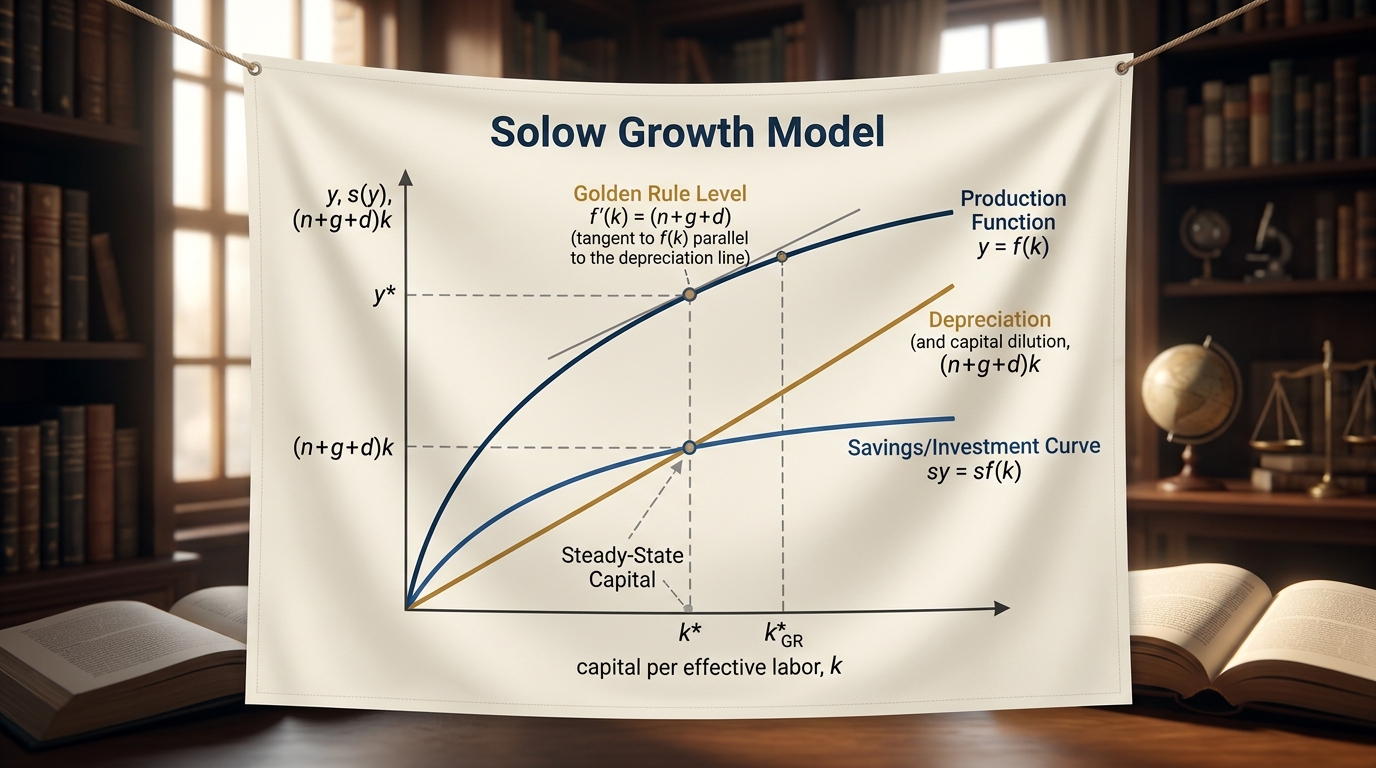
Solow Growth Model: Steady State, Golden Rule of Capital & Exam Numericals
Comprehensive 4,000-word masterclass on the Solow-Swan Neoclassical Growth Model for DU Economics students. Covers capital accumulation, steady state k*, Golden Rule level k*gold, technological progress, and 3 fully worked examination numericals.
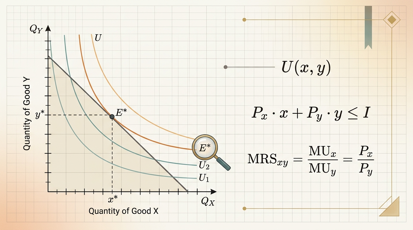
Consumer Theory & Indifference Curves: Utility Maximization, Budget Constraints & Exam Numericals
Comprehensive 4,000-word masterclass on Consumer Theory for DU Economics students. Covers utility functions, indifference curve properties, MRS derivation, budget constraint geometry, Lagrangian optimization, and 3 fully worked numerical problems.