Oligopoly Models: Cournot, Bertrand & Stackelberg — Complete Derivations & DU Exam Numericals
Comprehensive 4,000-word masterclass on Oligopoly Models for DU Economics students. Covers Cournot quantity competition, Bertrand price competition, Stackelberg leader-follower equilibrium, and 3 step-by-step worked numerical problems.

Oligopoly — a market structure dominated by a small number of strategically interdependent firms — is one of the most analytically rich topics in intermediate microeconomics. Unlike perfect competition or monopoly, oligopoly models require game-theoretic reasoning because each firm's optimal decision depends on what it expects its rivals to do.
For Delhi University B.A. (Hons) Economics students studying Intermediate Microeconomics I & II, oligopoly models consistently appear as 15-mark to 20-mark compulsory numerical questions. In this 4,000-word masterclass, we derive the equilibrium outcomes for the three canonical oligopoly models — Cournot (simultaneous quantity), Bertrand (simultaneous price), and Stackelberg (sequential quantity) — and solve 3 complete step-by-step examination numericals.
1. Market Structure Spectrum
| Feature | Perfect Competition | Oligopoly | Monopoly |
|---|---|---|---|
| Number of Firms | Very large (infinite) | Few (2 to ~10) | One |
| Strategic Interaction | None (price taker) | Central feature | None (sole producer) |
| Price | P = MC | MC < P < P_monopoly | MR = MC, P > MC |
| Output | Q_competitive (highest) | Q_monopoly < Q_oligopoly < Q_competitive | Q_monopoly (lowest) |
2. The Cournot Model (Simultaneous Quantity Competition)
Developed by Antoine Augustin Cournot (1838), this model assumes firms simultaneously choose output quantities, taking rivals' quantities as given.
2.1 Setup & Derivation
Consider a duopoly with inverse demand P = a - b*Q where Q = q1 + q2. Both firms have identical constant marginal cost c (no fixed costs).
Firm 1's Profit Maximization:
First-Order Condition (FOC): Take derivative with respect to q1 and set equal to 0:
Solving for q1 gives Firm 1's Best Response Function (Reaction Function):
By symmetry, Firm 2's Best Response is:
2.2 Cournot-Nash Equilibrium
At equilibrium, both reaction functions are satisfied simultaneously. By symmetry, q1* = q2*:
Total Q* = 2*(a - c) / (3*b)
P* = a - b * Q* = (a + 2*c) / 3
2.3 Generalization to N Firms
With N symmetric Cournot competitors:
Q* = N * (a - c) / [b*(N + 1)]
P* = (a + N*c) / (N + 1)
As N approaches infinity, P* approaches c and Q* approaches (a - c) / b — the perfectly competitive outcome.
3. The Bertrand Model (Simultaneous Price Competition)
Joseph Bertrand (1883) argued that firms compete on price rather than quantity. With homogeneous products and equal marginal costs, Bertrand competition yields a dramatically different result.
3.1 The Bertrand Paradox
If both firms produce identical goods and consumers buy from the cheapest supplier:
- If p1 > p2: Firm 1 sells nothing, Firm 2 captures entire market.
- If p1 = p2: Market is split equally.
- If p1 < p2: Firm 1 captures entire market.
Each firm has an incentive to undercut the rival by an infinitesimal amount. This undercutting spiral continues until:
Profit_1 = Profit_2 = 0
The Bertrand Paradox: With just 2 firms, the market achieves the perfectly competitive outcome (P = MC, zero economic profits). This is paradoxical because we would expect firms with market power to earn positive profits.
3.2 Escaping the Bertrand Paradox
- Product Differentiation: If goods are not perfect substitutes (e.g., Coca-Cola vs Pepsi), firms can sustain P > MC.
- Capacity Constraints: If firms cannot serve the entire market (Edgeworth model), undercutting to MC is not sustainable.
- Repeated Interaction: In infinitely repeated games, firms can sustain tacit collusion above MC.
4. The Stackelberg Model (Sequential Quantity Leadership)
Heinrich von Stackelberg (1934) modified Cournot by introducing sequential moves: Firm 1 (the Leader) moves first, and Firm 2 (the Follower) observes the leader's quantity before choosing its own.
4.1 Backward Induction Solution
Step 1: Solve for the Follower's Best Response (same as Cournot):
Step 2: Substitute into Leader's Profit Function:
= [a - b*q1 - (a - c)/2 + b*q1/2 - c] * q1
= [(a - c)/2 - b*q1/2] * q1
FOC:
Step 3: Follower's Equilibrium Quantity:
4.2 Key Stackelberg Results
| Variable | Cournot | Stackelberg |
|---|---|---|
| Leader Output | (a-c) / (3b) | (a-c) / (2b) — Higher |
| Follower Output | (a-c) / (3b) | (a-c) / (4b) — Lower |
| Total Output | 2(a-c) / (3b) | 3(a-c) / (4b) — Higher |
| Market Price | (a+2c) / 3 | (a+3c) / 4 — Lower |
First-Mover Advantage: The Stackelberg leader earns higher profit than the follower because committing to a large quantity first forces the follower to accommodate by producing less.
5. Worked Examination Numerical Problems
Numerical 1: Cournot Duopoly with Asymmetric Costs (15 Marks)
Question: Market demand is P = 120 - Q. Firm 1 has MC = 20, Firm 2 has MC = 30. Find Cournot equilibrium quantities, price, and profits.
Solution:
Firm 1's BR: q1 = (120 - 20 - q2) / 2 = 50 - q2/2
Firm 2's BR: q2 = (120 - 30 - q1) / 2 = 45 - q1/2
Substitute q2 into q1's BR:
3q1/4 = 27.5 ==> q1* = 36.67
Q* = 63.33, P* = 120 - 63.33 = 56.67
Profit_1 = (56.67 - 20) * 36.67 = 1,344.49
Profit_2 = (56.67 - 30) * 26.67 = 711.29
Numerical 2: Stackelberg with Linear Demand (15 Marks)
Question: P = 200 - 2Q, MC = 40 for both firms. Firm 1 is the Stackelberg leader. Find equilibrium.
Solution:
Follower's BR: q2 = (200 - 40)/(2*2) - q1/2 = 40 - q1/2
Leader substitutes:
q2_F = 40 - 40/2 = 20
Q* = 60, P* = 200 - 120 = 80
Profit_Leader = (80 - 40)*40 = 1,600
Profit_Follower = (80 - 40)*20 = 800
6. Summary Comparison & Exam Tips
- Cournot: Firms compete on quantity simultaneously. Output between monopoly and perfect competition.
- Bertrand: Firms compete on price. With identical products, P = MC (the paradox).
- Stackelberg: Sequential quantity. Leader produces more, earns more (first-mover advantage).
- Always show complete reaction function derivation in DU exams for full marks.
For related microeconomics guides, see our Game Theory & Nash Equilibrium Guide and Consumer Theory & Indifference Curves.
Frequently asked questions
Why is the Bertrand outcome called a paradox?
Because with just 2 firms, price competition drives the equilibrium to P = MC with zero economic profits — the same as perfect competition with infinitely many firms.
Does the Stackelberg leader always earn more than the follower?
Yes, with linear demand and identical costs, the leader's first-mover commitment to higher output forces the follower to produce less, giving the leader higher profit.
Dhairya sat the same DU papers he now writes about. Acadly is his attempt to say the useful things his own first-year self would have wanted to hear.
Keep reading
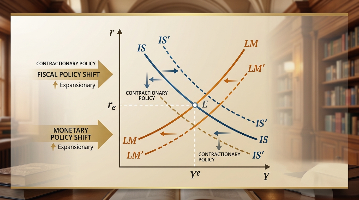
IS-LM Model: Goods & Money Market Equilibrium, Policy Multipliers & DU Exam Numericals
Comprehensive 4,000-word masterclass on the IS-LM model for DU Economics students. Covers algebraic derivations of IS and LM curves, general equilibrium, fiscal and monetary policy multipliers, crowding-out effect, liquidity trap, and 3 fully worked exam numericals.
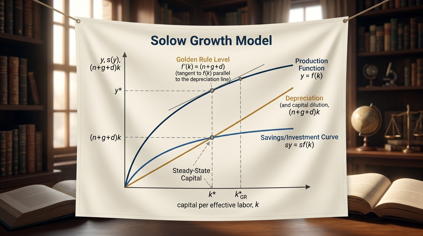
Solow Growth Model: Steady State, Golden Rule of Capital & Exam Numericals
Comprehensive 4,000-word masterclass on the Solow-Swan Neoclassical Growth Model for DU Economics students. Covers capital accumulation, steady state k*, Golden Rule level k*gold, technological progress, and 3 fully worked examination numericals.
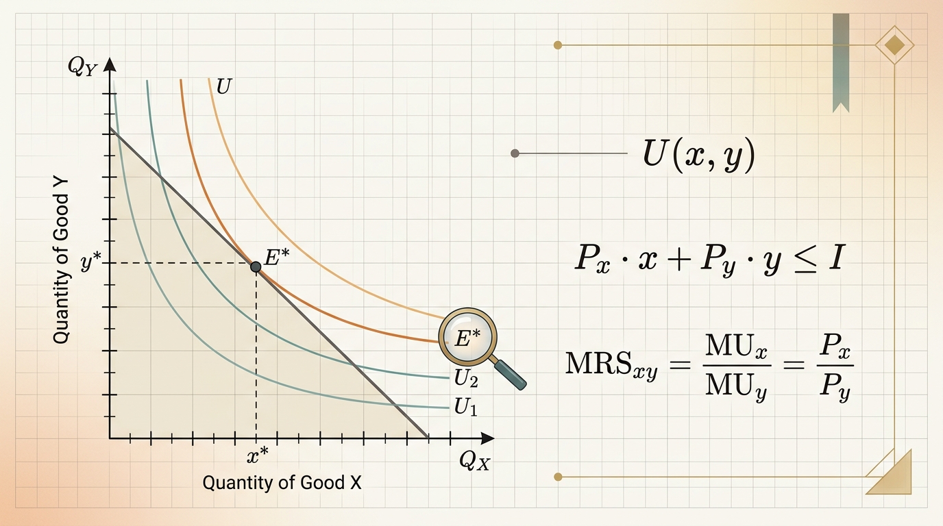
Consumer Theory & Indifference Curves: Utility Maximization, Budget Constraints & Exam Numericals
Comprehensive 4,000-word masterclass on Consumer Theory for DU Economics students. Covers utility functions, indifference curve properties, MRS derivation, budget constraint geometry, Lagrangian optimization, and 3 fully worked numerical problems.