Consumer Theory & Indifference Curves: Utility Maximization, Budget Constraints & Exam Numericals
Comprehensive 4,000-word masterclass on Consumer Theory for DU Economics students. Covers utility functions, indifference curve properties, MRS derivation, budget constraint geometry, Lagrangian optimization, and 3 fully worked numerical problems.
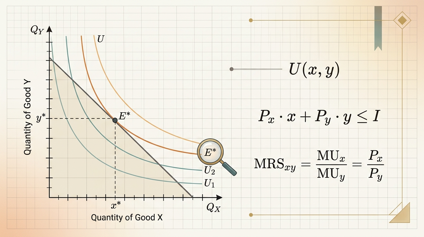
Consumer Theory is the foundational pillar of microeconomics. It explains how rational consumers allocate their limited income across goods and services to achieve maximum satisfaction (utility). For Delhi University B.A. (Hons) Economics students, Consumer Theory dominates Semester 1 Introductory Microeconomics and Semester 3 Intermediate Microeconomics I, appearing consistently as 15-mark and 20-mark exam questions.
In this 4,000-word numerical masterclass, we derive the mathematical properties of utility functions, prove indifference curve convexity, derive the Marginal Rate of Substitution (MRS), set up the Lagrangian constrained optimization framework, solve for Marshallian and Hicksian demand functions, and work through 3 complete step-by-step examination numerical problems.
1. The Utility Function
A utility function U(x1, x2) assigns a numerical value to each consumption bundle (x1, x2) representing the consumer's preference ordering. If Bundle A is preferred to Bundle B, then U(A) > U(B).
1.1 Properties of Well-Behaved Preferences
- Completeness: For any two bundles A and B, either A is preferred to B, B is preferred to A, or the consumer is indifferent.
- Transitivity: If A is preferred to B, and B is preferred to C, then A is preferred to C.
- Non-Satiation (Monotonicity): More of any good is always (weakly) preferred. If bundle A has more of at least one good and no less of any other, A is preferred to B.
- Convexity: Averages are preferred to extremes. If the consumer is indifferent between A and B, then any weighted average t*A + (1-t)*B (where 0 < t < 1) is at least as good as A or B.
1.2 Common Utility Function Forms
| Utility Type | Functional Form | IC Shape | MRS Property |
|---|---|---|---|
| Cobb-Douglas | U = x1^a * x2^b | Smooth, strictly convex hyperbolas | Diminishing MRS |
| Perfect Substitutes | U = a*x1 + b*x2 | Straight lines with slope -a/b | Constant MRS = a/b |
| Perfect Complements (Leontief) | U = min(a*x1, b*x2) | L-shaped with kink at a*x1 = b*x2 | MRS undefined at kink; 0 or infinity elsewhere |
| Quasi-Linear | U = v(x1) + x2 | Vertically parallel curves | MRS depends only on x1 |
2. Indifference Curves: Definition & Properties
An indifference curve is the locus of all consumption bundles that yield the same level of utility. Formally, for a given utility level u_bar, the indifference curve is:
2.1 Five Key Properties of Indifference Curves
- Downward Sloping: By non-satiation, if x1 increases, x2 must decrease to maintain the same utility. Hence ICs slope downward.
- Higher ICs Represent Greater Utility: By monotonicity, a bundle on a higher IC (farther from origin) is strictly preferred.
- ICs Cannot Intersect: If two ICs intersected at a point, transitivity would be violated. Proof: Suppose IC1 and IC2 cross at point P. Take point A on IC1 and point B on IC2 (different from P). Then A ~ P (same IC1), and B ~ P (same IC2), so by transitivity A ~ B. But A is on a different IC than B, implying different utility — contradiction.
- ICs Are Thin: Each IC has zero thickness (it is a curve, not a band).
- Convex to the Origin: By the convexity axiom, ICs bow inward toward the origin, reflecting diminishing MRS.
3. Marginal Rate of Substitution (MRS)
The MRS measures the rate at which a consumer is willing to trade Good 2 for Good 1 while maintaining the same utility level. It equals the (negative of the) slope of the indifference curve.
3.1 Derivation via Total Differential
Along an indifference curve, utility is constant: dU = 0. Taking the total differential of U(x1, x2):
Rearranging:
where MU1 = dU/dx1 is the marginal utility of Good 1, and MU2 = dU/dx2 is the marginal utility of Good 2.
3.2 Diminishing MRS
For well-behaved (strictly convex) preferences, the MRS diminishes as x1 increases along an IC. Intuitively, as you accumulate more of Good 1, each additional unit becomes less valuable relative to Good 2, so you are willing to give up less of Good 2 per unit of Good 1.
4. The Budget Constraint
A consumer with income M faces prices p1 and p2 for goods 1 and 2. The budget constraint defines the affordable set:
The budget line (where the constraint binds with equality) has slope -p1/p2, x1-intercept M/p1, and x2-intercept M/p2.
5. Utility Maximization: The Tangency Condition
The consumer chooses the bundle on the highest achievable IC that still satisfies the budget constraint. At the optimum (interior solution), the IC is tangent to the budget line:
This is the equi-marginal principle: at the optimum, the marginal utility per rupee spent is equalized across all goods.
5.1 Lagrangian Method
Set up the constrained optimization problem:
Lagrangian:
First-Order Conditions (FOCs):
dL/dx2 = MU2 - lambda*p2 = 0 ==> MU2 = lambda*p2
dL/dlambda = M - p1*x1 - p2*x2 = 0
Dividing the first FOC by the second: MU1/MU2 = p1/p2, which is the tangency condition. The Lagrange multiplier lambda represents the marginal utility of income.
6. Worked Examination Numerical Problems
Numerical Problem 1: Cobb-Douglas Utility Maximization (15 Marks)
Question: A consumer has utility function U(x1, x2) = x1^(1/3) * x2^(2/3). Prices are p1 = 4, p2 = 8, and income M = 240. Find the optimal consumption bundle and the maximum utility.
Solution:
Step 1: Find Marginal Utilities
MU2 = dU/dx2 = (2/3) * x1^(1/3) * x2^(-1/3)
Step 2: Apply Tangency Condition MU1/MU2 = p1/p2
= (1/3 * x2) / (2/3 * x1) = x2 / (2*x1)
Setting MRS = p1/p2 = 4/8 = 1/2:
Step 3: Substitute into Budget Constraint
4*x1 + 8*x1 = 240 (since x2 = x1)
12*x1 = 240
U* = 20^(1/3) * 20^(2/3) = 20
Verification (Expenditure Share Property): For Cobb-Douglas U = x1^a * x2^b, the income share spent on Good 1 is a/(a+b). Here a = 1/3, b = 2/3, so share on Good 1 = (1/3) / (1) = 1/3. Expenditure on x1 = 4 * 20 = 80 = 240/3. Correct!
Numerical Problem 2: Perfect Substitutes (10 Marks)
Question: A consumer has utility U = 3*x1 + 5*x2. Prices are p1 = 6, p2 = 10, and income M = 120. Find the optimal bundle.
Solution:
For perfect substitutes, the consumer compares MU1/p1 vs MU2/p2:
MU2/p2 = 5/10 = 0.5
Since MU1/p1 = MU2/p2, the consumer is indifferent between all bundles on the budget line. Any combination of x1 and x2 satisfying 6*x1 + 10*x2 = 120 is optimal.
Maximum Utility = 3*(120/6) = 60 (or 5*(120/10) = 60 — same!)
Numerical Problem 3: Income and Substitution Effects (20 Marks)
Question: A consumer has utility U = x1 * x2. Initially p1 = 2, p2 = 4, M = 80. Price of Good 1 falls to p1' = 1. Decompose the change in demand for x1 into Substitution Effect and Income Effect using the Slutsky method.
Solution:
Step 1: Find Initial Optimal Bundle (A)
For U = x1 * x2 (Cobb-Douglas with a = b = 1), optimal demands are:
x2* = M/(2*p2) = 80/(2*4) = 10
Bundle A = (20, 10)
Step 2: Find Final Optimal Bundle (C) after price change
x2** = M/(2*p2) = 80/(2*4) = 10
Bundle C = (40, 10)
Step 3: Slutsky Decomposition — Find Compensated Income (M')
Slutsky compensation: M' = new prices * original bundle:
Step 4: Find Intermediate Bundle (B) at new prices with compensated income
Bundle B = (30, 7.5)
Step 5: Decompose Total Effect
Substitution Effect (A to B) = x1_B - x1* = 30 - 20 = +10 units
Income Effect (B to C) = x1** - x1_B = 40 - 30 = +10 units
Both effects are positive (Good 1 is a normal good): the price decrease makes it relatively cheaper (substitution effect) and increases real purchasing power (income effect).
7. Summary Checklist for DU Exams
- Always state the tangency condition MRS = p1/p2 before solving.
- For Cobb-Douglas, use the expenditure share shortcut to verify answers.
- For perfect substitutes, compare MU/p ratios — corner solutions are typical.
- For perfect complements, set a*x1 = b*x2 and substitute into the budget constraint.
- In Slutsky decomposition, always clearly label Bundles A, B, and C.
For related microeconomics guides, see our Elasticity of Demand Masterclass and Game Theory & Nash Equilibrium Guide.
Frequently asked questions
Why can two indifference curves never intersect?
If two ICs crossed at point P, transitivity would be violated: bundles on different ICs (with different utility levels) would both be indifferent to P, implying they have equal utility — a contradiction.
What is the expenditure share shortcut for Cobb-Douglas utility?
For U = x1^a * x2^b, the consumer always spends fraction a/(a+b) of income on Good 1 and b/(a+b) on Good 2, regardless of prices.
Dhairya sat the same DU papers he now writes about. Acadly is his attempt to say the useful things his own first-year self would have wanted to hear.
Keep reading
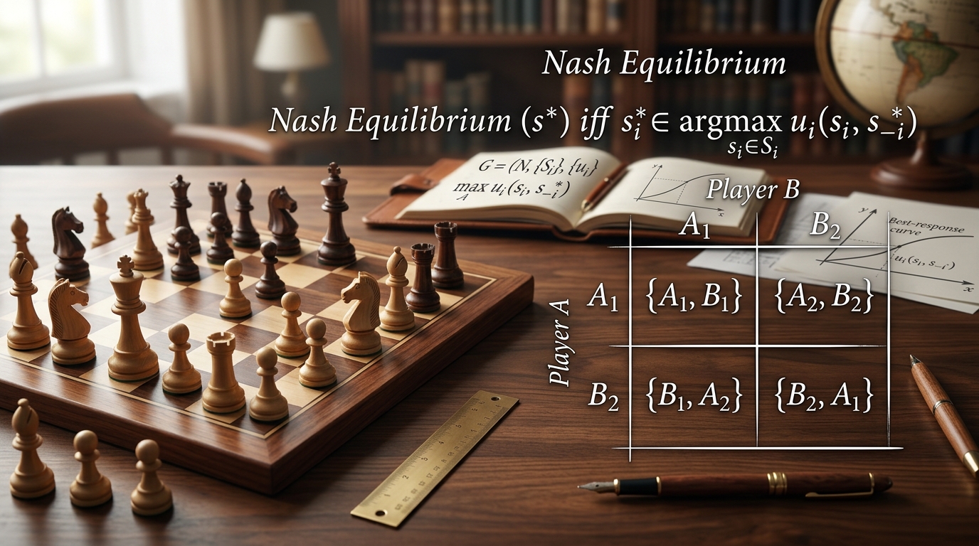
Game Theory & Nash Equilibrium: Mathematical Derivations, Payoff Matrices & Exam Numericals
Comprehensive 4,000-word masterclass on Game Theory and Nash Equilibrium for DU Economics students. Covers dominant strategies, Prisoner's Dilemma, mixed strategies, Cournot duopoly, and 3 fully worked numerical problems.
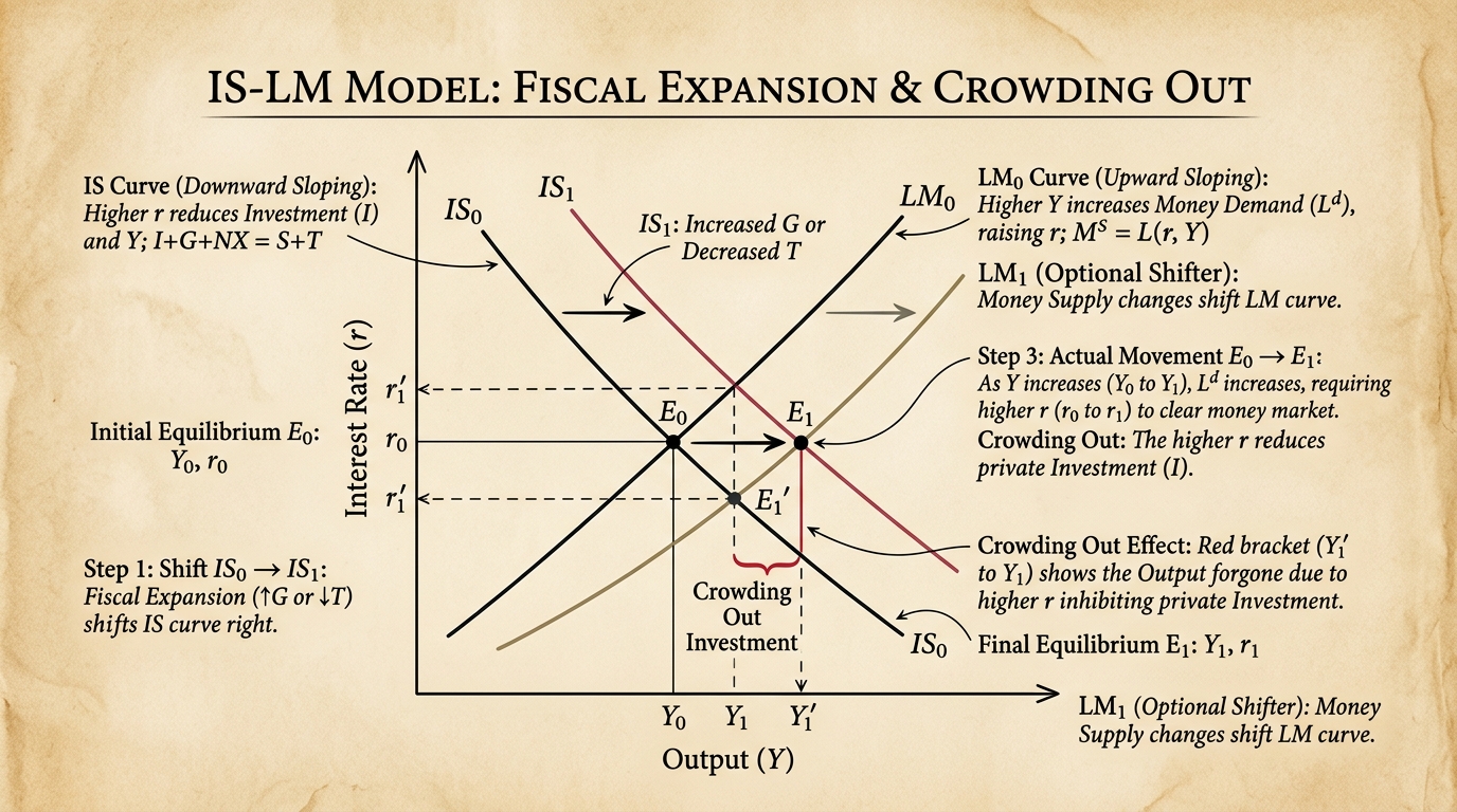
Mundell-Fleming Model: Fixed vs Floating Exchange Rates (Complete Derivations & Policy Efficacy)
Exhaustive 4,500-word masterclass on the Mundell-Fleming open economy macroeconomics model. Includes algebraic derivations of IS*, LM*, BP curves, Marshall-Lerner condition, and India's exchange rate policy.

Cobb-Douglas Production Function: Mathematical Properties, Homogeneity & Returns to Scale Proofs
Exhaustive 4,500-word mathematical masterclass on the Cobb-Douglas production function. Mathematical proofs of Euler's Theorem, constant/increasing returns to scale, marginal productivity, output elasticity, and expansion paths.