Mundell-Fleming Model: Fixed vs Floating Exchange Rates (Complete Derivations & Policy Efficacy)
Exhaustive 4,500-word masterclass on the Mundell-Fleming open economy macroeconomics model. Includes algebraic derivations of IS*, LM*, BP curves, Marshall-Lerner condition, and India's exchange rate policy.
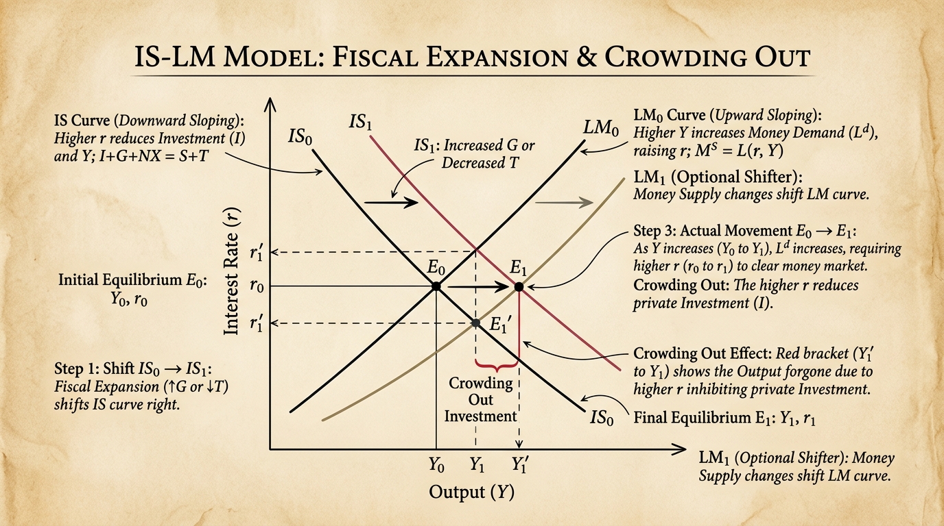
The Mundell-Fleming model represents the bedrock of open-economy macroeconomics. As an extension of the IS-LM framework, it describes the short-run relationship between an economy's nominal exchange rate, interest rate, and output. For advanced macroeconomics students—particularly those navigating university curricula across India—mastering the algebraic derivations of the IS*, LM*, and BP curves is mandatory. This comprehensive guide provides step-by-step proofs, policy efficacy analyses under both Fixed and Floating exchange rate regimes, the J-Curve effect, and the realities of India's exchange rate policy spanning from 2000 to 2026.
1. Algebraic Derivations: IS*, LM*, and BP Curves
The IS* Curve: Goods Market Equilibrium
The IS* curve represents equilibrium in the open-economy goods market. National Income (Y) equals Consumption (C), Investment (I), Government Spending (G), and Net Exports (NX). In an open economy, Net Exports depend on the real exchange rate (e) and output (Y).
Y = C(Y - T) + I(r) + G + NX(e, Y*)
Assuming a linear framework:
C = c0 + c1(Y - T) where c1 is marginal propensity to consume.
I = I0 - b(r) where b measures interest sensitivity of investment.
NX = X0 - m(Y) - v(e) where m is marginal propensity to import, v is sensitivity of net exports to exchange rate.
Substitute these into the national income identity:
Y = c0 + c1(Y - T) + I0 - b(r) + G + X0 - m(Y) - v(e)
Y - c1(Y) + m(Y) = c0 - c1(T) + I0 + G + X0 - b(r) - v(e)
Y (1 - c1 + m) = [c0 - c1(T) + I0 + G + X0] - b(r) - v(e)
Let A_bar = c0 - c1(T) + I0 + G + X0 (Autonomous Spending)
Y = [ A_bar - b(r) - v(e) ] / (1 - c1 + m)
Notice that the IS* curve slopes downward with respect to the exchange rate (e). A higher exchange rate (currency appreciation) reduces net exports, lowering equilibrium output Y.
The LM* Curve: Money Market Equilibrium
The LM* curve represents equilibrium in the money market. Real money supply (M/P) equals real money demand (L), which depends on income (Y) and the domestic interest rate (r). Under perfect capital mobility, the domestic interest rate equals the world interest rate (r = r*).
M / P = L(r*, Y)
Assuming a linear money demand function:
M / P = k(Y) - h(r*)
k(Y) = M / P + h(r*)
Y = (1/k) [ M / P + h(r*) ]
Because r is pegged to r*, the LM* curve is a vertical line when plotted in a (Y, e) space. It determines the equilibrium level of income independently of the exchange rate, strictly based on the real money supply.
The BP Curve: Balance of Payments Equilibrium
The BP (Balance of Payments) curve traces the combinations of interest rates and output where the overall balance of payments is zero. BP = Current Account (CA) + Capital Account (KA) = 0.
CA = NX(e, Y) = X0 - m(Y) - v(e)
KA = f(r - r*) where f is the degree of capital mobility.
BP = CA + KA = X0 - m(Y) - v(e) + f(r - r*) = 0
- Perfect Capital Mobility (f approaches infinity): Even a tiny deviation of r from r* causes massive capital flows. The BP curve is a horizontal line at r = r*.
- Imperfect Capital Mobility: The BP curve is upward sloping. Higher Y causes a trade deficit, requiring a higher r to attract capital and balance payments.
- Zero Capital Mobility (f = 0): The BP curve is a vertical line at the income level where NX = 0.
2. Policy Effectiveness Proofs (Perfect Capital Mobility)
Fiscal Policy under Fixed Exchange Rates (Highly Effective)
Suppose the government increases spending (Delta G > 0).
- The IS* curve shifts to the right, pushing the domestic interest rate r above r*.
- r > r* triggers a massive capital inflow, putting upward pressure on the domestic currency.
- To maintain the fixed exchange rate peg, the central bank must intervene by selling domestic currency and buying foreign assets.
- This intervention increases the money supply (M).
- The LM* curve shifts to the right until r is pushed back down to r*.
- Result: Fiscal policy is highly effective. Income Y increases fully by the multiplier effect, with no crowding out. Delta Y = Multiplier × Delta G.
Monetary Policy under Floating Exchange Rates (Highly Effective)
Suppose the central bank increases the money supply (Delta M > 0).
- The LM* curve shifts to the right, pushing the domestic interest rate r below r*.
- r < r* triggers a massive capital outflow, putting downward pressure on the domestic currency.
- Under a floating regime, the currency depreciates (e decreases).
- A lower e stimulates Net Exports (NX increases).
- The IS* curve shifts rightward along the new LM* curve.
- Result: Monetary policy is highly effective. Income Y increases, entirely driven by the boost in net exports rather than domestic investment.
3. Three Fully Worked Numerical Problems
Problem 1: Equilibrium in Floating Regime
Given: C = 100 + 0.8(Y - T), I = 200 - 10r, G = 150, T = 100. NX = 100 - 0.1Y - 10e. M/P = Y - 20r. World interest rate r* = 5.
Find: Equilibrium Y and e.
1. Find LM* equilibrium (Y):
Since perfect capital mobility, r = r* = 5.
Suppose M/P is set by Central Bank at 800.
800 = Y - 20(5) => 800 = Y - 100 => Y = 900.
2. Find IS* equilibrium (e):
Y = C + I + G + NX
900 = [100 + 0.8(900 - 100)] + [200 - 10(5)] + 150 + [100 - 0.1(900) - 10e]
900 = [100 + 0.8(800)] + [150] + 150 + [100 - 90 - 10e]
900 = [100 + 640] + 150 + 150 + [10 - 10e]
900 = 740 + 300 + 10 - 10e
900 = 1050 - 10e
10e = 150 => e = 15.
Problem 2: Fiscal Expansion under Fixed Peg
Given: Same equations, but e is fixed at 15. The government increases G from 150 to 200 (Delta G = 50).
Find: New Y and the necessary Delta M to maintain the peg.
1. Since e=15 and r=5 are fixed, solve IS for new Y:
Y = 100 + 0.8(Y - 100) + 200 - 10(5) + 200 + 100 - 0.1Y - 10(15)
Y = 100 + 0.8Y - 80 + 150 + 200 + 100 - 0.1Y - 150
Y = 320 + 0.7Y
0.3Y = 320 => Y = 320 / 0.3 = 1066.67
2. Determine required M/P:
M/P = Y - 20r
M/P = 1066.67 - 20(5) = 1066.67 - 100 = 966.67
Initial M/P was 800. Delta M/P = 166.67.
The central bank must increase money supply by 166.67 to prevent currency appreciation and maintain e=15.
4. The Marshall-Lerner Condition and the J-Curve
The Mundell-Fleming model assumes that a currency depreciation improves the trade balance (NX increases as e decreases). This holds true only if the Marshall-Lerner Condition is satisfied.
The condition states that a real depreciation improves the trade balance if the sum of the price elasticities of demand for exports (E_x) and imports (E_m) is greater than 1:
|E_x| + |E_m| > 1
In the short run, elasticities are often low due to pre-existing contracts and lag in consumer behavior. This leads to the J-Curve Effect: an immediate deterioration of the trade balance post-depreciation (as import prices rise instantly in domestic terms), followed by an improvement over the medium-to-long term as volumes adjust.
5. The Impossible Trinity & India's Exchange Rate Policy (2000-2026)
The Mundell-Fleming framework mathematically proves the Impossible Trinity (Trilemma). A nation cannot simultaneously achieve:
- Free Capital Mobility
- A Fixed Exchange Rate
- Independent Monetary Policy
| Country / Region | Sacrificed Goal | Real-World Execution |
|---|---|---|
| USA | Fixed Exchange Rate | Fully floating USD, free capital mobility, Federal Reserve sets rates independently. |
| Eurozone Members | Independent Monetary Policy | Fixed rates (common Euro currency), free capital flows. The ECB dictates policy. |
| China | Free Capital Mobility | Managed peg, PBOC sets rates, but maintains strict capital controls to prevent flight. |
| India (2000-2026) | Hybrid / Managed Float | RBI intervenes to smooth volatility, controls on speculative debt flows, independent repo rate. |
India's approach is often termed a "managed float" or "dirty float." Rather than sacrificing one pillar entirely, the RBI maintains a middle ground. India allows significant FDI and FPI flows but restricts certain external commercial borrowings (imperfect capital mobility). This allows the RBI to maintain a somewhat independent monetary policy while preventing excessive INR volatility against the USD.
6. Expand Your Micro & Macro Knowledge
Connecting macro concepts with microfoundations gives a holistic view of the economy. If you enjoyed this derivation, be sure to study the foundational microeconomic proofs in our Cobb-Douglas Production Function Masterclass.
Are you an undergraduate preparing your semester strategy? Learn how to pick the best non-core papers by reading our 2026 DU GE, SEC, and VAC Course Selection Guide, and track your resulting grades flawlessly with our SGPA to CGPA Calculation framework. Finally, if you aim to utilize these macro models in top-tier research, check out the career pathways in our IGIDR vs DSE Comparison Guide.
Frequently asked questions
Why is fiscal policy ineffective under floating exchange rates?
Because increased interest rates cause currency appreciation, crowding out net exports completely.
Dhairya sat the same DU papers he now writes about. Acadly is his attempt to say the useful things his own first-year self would have wanted to hear.
Keep reading
Consumer Theory & Indifference Curves: Utility Maximization, Budget Constraints & Exam Numericals
Comprehensive 4,000-word masterclass on Consumer Theory for DU Economics students. Covers utility functions, indifference curve properties, MRS derivation, budget constraint geometry, Lagrangian optimization, and 3 fully worked numerical problems.

Game Theory & Nash Equilibrium: Mathematical Derivations, Payoff Matrices & Exam Numericals
Comprehensive 4,000-word masterclass on Game Theory and Nash Equilibrium for DU Economics students. Covers dominant strategies, Prisoner's Dilemma, mixed strategies, Cournot duopoly, and 3 fully worked numerical problems.

Cobb-Douglas Production Function: Mathematical Properties, Homogeneity & Returns to Scale Proofs
Exhaustive 4,500-word mathematical masterclass on the Cobb-Douglas production function. Mathematical proofs of Euler's Theorem, constant/increasing returns to scale, marginal productivity, output elasticity, and expansion paths.