Introductory Microeconomics Unit 5: Perfect Competition, Short & Long Run Equilibrium Notes
Master DU Sem 1 Unit 5: Perfect competition assumptions, firm vs industry equilibrium, shutdown point P < AVC, short/long-run supply curve derivation & social efficiency.
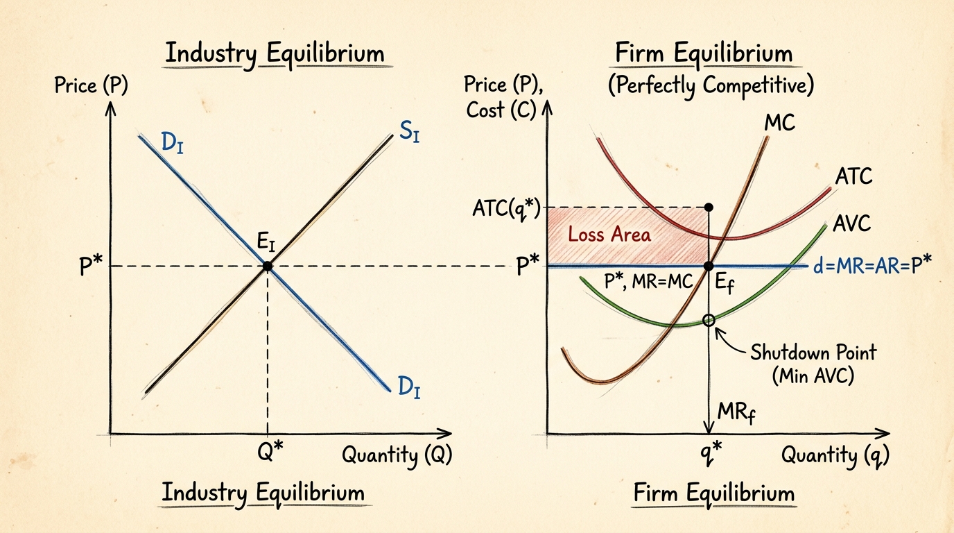
Welcome to Unit 5 of Introductory Microeconomics for Delhi University Semester 1! In this unit, we shift our focus from consumer and producer behavior to how they interact in the marketplace under Perfect Competition. This is a highly foundational chapter, building directly on the cost curves (Unit 4) and revenue concepts you've previously learned.
This massive, comprehensive guide is designed to act as your complete replacement for reading hefty textbooks, offering clear explanations, real-world Indian examples, step-by-step mathematical derivations, graphical intuition, and past year question frameworks. Let's dive deep into Perfect Competition, Firm vs Industry Equilibrium, Supply Curve derivation, and Efficiency analysis.
1. Features & Assumptions of Perfect Competition
Perfect competition is a theoretical market structure. While it rarely exists in its absolute pure form, markets like agricultural commodities (wheat, rice in an APMC mandi) or stock markets come very close. It serves as a benchmark against which all other market structures (Monopoly, Monopolistic Competition, Oligopoly) are judged.
Key Characteristics
- Large Number of Buyers and Sellers: The market is highly atomistic. No single buyer or seller is large enough to influence the market price. The share of a single firm's output in the total industry output is mathematically negligible.Result: Every firm is a Price Taker. They must accept the prevailing market price determined by industry demand and supply.
- Homogeneous Product: Every firm produces a product that is perfectly identical (perfect substitute) to the product of every other firm in terms of physical characteristics, quality, branding, etc.Result: If a firm raises its price even slightly above the market price, its sales will drop to zero because consumers will instantly switch to competitors.
- Free Entry and Exit: Firms can enter the industry if they see supernormal profits and can leave if they incur losses, without any significant barriers (legal, technical, or financial). This is particularly crucial for Long-Run Equilibrium.
- Perfect Knowledge: Both buyers and sellers have complete information about prices, technology, and costs. There are no information asymmetries.
- Perfect Mobility of Factors of Production: Labor and capital can move freely between firms and industries in search of the highest returns.
- Absence of Transport Costs: Assumed to simplify the model, ensuring the price remains identical everywhere.
The Firm's Demand Curve (Price Taker Condition)
Because the firm is a price taker, it can sell any quantity of output at the prevailing market price, say P*. Therefore, the demand curve facing an individual firm is perfectly elastic (a horizontal straight line) at the market price level.
Mathematically, Total Revenue (TR) = P * Q.
Average Revenue (AR) = TR / Q = (P * Q) / Q = P.
Marginal Revenue (MR) = d(TR) / dQ = P (since P is constant).
Conclusion: For a perfectly competitive firm, P = AR = MR. The horizontal demand curve is also the AR and MR curve.
2. Short-Run Equilibrium of a Competitive Firm
In the short run, at least one factor of production (usually capital) is fixed. Firms cannot enter or exit the industry; the number of firms is fixed. The firm’s objective is to maximize its economic profit (Pi), where Pi = TR - TC.
Profit Maximization Rules (MR-MC Approach)
Instead of looking at total curves, economists prefer marginal analysis. The firm achieves equilibrium (maximum profit) when two conditions are met:
- Necessary Condition (First Order): MR = MC. If MR > MC, producing an extra unit adds more to revenue than to cost, increasing profit. If MR < MC, producing an extra unit decreases profit. Hence, profits are maximized when MR = MC. Since MR = P, the rule becomes P = MC.
- Sufficient Condition (Second Order): MC curve must cut the MR curve from below. This means MC must be rising at the point of equilibrium (Slope of MC > 0). If MC cuts MR from above, it's a point of profit minimization.
Three Short-Run Scenarios
Depending on the position of the Short-Run Average Cost (SAC) relative to Price (AR), a firm can face three situations in the short run:
- Supernormal (Economic) Profit: If at equilibrium quantity Q*, the Price (P*) > SAC. The firm covers all its explicit and implicit costs and makes an extra profit. Profit = (AR - SAC) * Q*. The profit area is a rectangle between the price line and SAC curve.
- Normal Profit (Zero Economic Profit): If at Q*, Price (P*) = SAC. The firm just covers its total economic costs. TR = TC. The SAC curve is exactly tangent to the AR=MR line at the minimum point of SAC.
- Subnormal Profit (Economic Loss): If at Q*, Price (P*) < SAC. The firm's revenue is less than its total cost. Loss = (SAC - AR) * Q*. But does the firm shut down immediately? Not necessarily! This leads us to the shutdown point.
3. Shutdown Decision & Derivation of Short-Run Supply Curve
A key concept in DU exams is the firm's decision to continue producing or shut down when making losses.
The Shutdown Rule
In the short run, Total Cost (TC) = Total Fixed Cost (TFC) + Total Variable Cost (TVC). Even if the firm produces zero units (shuts down), it still has to pay TFC (rent, insurance, etc.). These are often considered "sunk costs" in the short run. Therefore, if the firm shuts down, its Loss = TFC.
If the firm produces, its Loss = TC - TR = (TFC + TVC) - TR. The firm will choose the option that minimizes its losses. It will continue to produce as long as TR > TVC, or dividing by Q, as long as P > AVC (Average Variable Cost).
The Shutdown Point: This occurs where Price equals the minimum of Average Variable Cost (P = min AVC). At this point, TR = TVC. The firm is indifferent between producing and shutting down because its loss equals TFC in both cases. If price falls even a fraction of a rupee below min AVC, the firm shuts down, producing Q = 0.
Deriving the Short-Run Supply Curve
The firm's supply curve shows the quantity it will supply at various prices. Since the firm always sets P = MC (as long as it produces), the MC curve tells us the quantity supplied at any given price.
However, the firm will not supply anything if P < min AVC.Conclusion: The short-run supply curve of a perfectly competitive firm is the portion of its Marginal Cost (MC) curve that lies above the minimum point of the Average Variable Cost (AVC) curve. For prices below min AVC, the quantity supplied is zero.
4. Industry Short-Run Supply Curve
The short-run market (industry) supply curve is derived by taking the horizontal summation of the short-run supply curves (the MC curves above min AVC) of all individual firms in the industry.
If there are 100 identical firms, and at Price = Rs 20, one firm supplies 50 units, the industry supplies 100 * 50 = 5000 units. Mathematically: Q_industry(P) = Summation(i=1 to n) [q_i(P)].
The industry demand curve is downward sloping (Law of Demand). The intersection of the industry demand curve and the industry short-run supply curve determines the short-run equilibrium market price (P*).
5. Long-Run Equilibrium of Firm & Industry
In the long run, all factors of production are variable. Firms can alter their plant size, and crucially, new firms can enter the industry or existing ones can leave.
The Adjustment Process (Entry and Exit)
If firms in the industry are making supernormal profits in the short run, this acts as a magnet for new firms. As new firms enter, the industry supply curve shifts to the right. This increases total market quantity but drives the market price down. The price will continue to fall until supernormal profits are wiped out, i.e., until P = min LAC (Long-Run Average Cost).
Conversely, if firms are making losses, some firms will exit the industry over time. The industry supply curve shifts left, driving the market price up, until the remaining firms are making normal profits.
Long-Run Equilibrium Conditions
For the industry to be in long-run equilibrium, every firm must be making exactly zero economic profit (normal profit). The conditions are:
- Firms maximize long-run profit: P = LMC.
- Firms earn zero economic profit: P = LAC.
- Therefore, P = LMC = LAC. Since LMC intersects LAC at its minimum point, the firm operates at the minimum efficient scale.
Furthermore, in the long run, the firm's short-run curves also align perfectly. The grand equation for Long-Run Equilibrium of a perfectly competitive firm is:P = MR = AR = LMC = LAC = SMC = SAC(where SMC and SAC are the Short-Run Marginal and Average Cost curves for the optimal plant size).
Long-Run Industry Supply Curve (LS)
The shape of the long-run industry supply curve depends on how input prices react when the entire industry expands (due to new firm entry). We have three cases:
- Constant Cost Industry: As the industry expands, input prices (like raw materials, labor wages) remain unchanged. The new firms have the exact same cost curves as the old ones. The long-run supply (LS) curve is a horizontal line at the price equal to min LAC.
- Increasing Cost Industry: (Most common). As the industry expands, the increased demand for inputs drives up input prices. Cost curves of all firms shift upward. The new equilibrium price must be higher to cover the higher minimum LAC. The LS curve is upward sloping. Example: Agricultural land becoming scarce as farming expands.
- Decreasing Cost Industry: As the industry expands, it creates positive external economies of scale (e.g., a localized hub forms, leading to cheaper specialized labor or better infrastructure). Input prices fall, shifting cost curves down. The LS curve is downward sloping. Example: Early days of the tech hardware industry.
6. Efficiency Analysis: Why Perfect Competition is "Perfect"
Economists love perfect competition because, under certain assumptions, it leads to the optimal allocation of society's scarce resources.
Allocative Efficiency (P = MC)
Allocative efficiency occurs when resources are allocated to produce the exact mix of goods that society values most. Price (P) represents the marginal benefit to society of consuming one more unit. Marginal Cost (MC) represents the opportunity cost to society of producing that unit. In perfect competition, since firms set P = MC, the marginal benefit equals marginal cost. No one can be made better off without making someone else worse off (Pareto Optimality).
Productive Efficiency (P = min LAC)
Productive efficiency occurs when goods are produced at the lowest possible cost. In long-run perfect competition, firms are forced to produce at the minimum point of their Long-Run Average Cost (LAC) curve to survive. No resources are wasted.
Maximization of Total Social Surplus
Total Surplus = Consumer Surplus (CS) + Producer Surplus (PS). In a perfectly competitive market left to itself (no government intervention, no externalities), the equilibrium price and quantity maximize the total surplus area. Any interference (like a price floor or ceiling) will create a Deadweight Loss (DWL).
7. Impact of Taxes & Subsidies
Understanding how government intervention affects the competitive equilibrium is a favorite DU exam topic.
Per-Unit Tax (Specific Tax)
- Short Run: A tax of 't' per unit shifts the firm's MC and AVC curves upward by 't'. The industry supply curve shifts upward by 't'. Result: Market price rises (but usually by less than 't'), quantity exchanged falls. Consumer and Producer surplus fall, creating deadweight loss. Firms may make short-run losses.
- Long Run: In a constant cost industry, the long-run supply curve shifts up by exactly 't'. The entire burden of the tax is passed on to consumers. Price rises by 't', firms return to normal profit (zero economic profit), and industry output shrinks as some firms exit.
Lump-Sum Tax
- Short Run: A fixed lump-sum tax (like a license fee) affects only Total Fixed Cost (TFC) and Average Fixed Cost (AFC). It does NOT change Marginal Cost (MC) or Average Variable Cost (AVC). Therefore, the firm's short-run profit-maximizing quantity (where P = MC) remains completely unchanged. The firm just absorbs the tax out of its profits. It does not affect the industry supply or price in the short run.
- Long Run: The lump-sum tax increases Average Cost (AC). Firms now make losses and exit the industry. Industry supply shifts left, raising the market price until remaining firms cover the higher AC. The lump-sum tax acts like a fixed cost that eventually gets passed to consumers.
8. Fully Solved Numericals for DU Exams
Let's tackle the heavy-hitting numericals that carry 6-8 marks in your final exams.
Numerical 1: Profit Maximization and Shutdown Point
Question: A perfectly competitive firm has a Total Cost function given by: TC = 0.5Q^2 + 10Q + 50. The market price is P = 40.
a) Find the profit-maximizing output (Q*).
b) Calculate the maximum profit.
c) Find the minimum price required for the firm to avoid shutting down in the short run.
Solution:
Part a) Output (Q*)
Rule for profit maximization: P = MC.
First, find MC by differentiating TC with respect to Q:
MC = d(TC)/dQ = d(0.5Q^2 + 10Q + 50)/dQ = 1.0Q + 10 = Q + 10.
Set P = MC:
40 = Q + 10
Q* = 30 units.
(Check second order: Slope of MC is d(MC)/dQ = 1 > 0. So it's a maximum).
Part b) Maximum Profit
Profit = TR - TC.
TR = P * Q = 40 * 30 = 1200.
TC = 0.5(30)^2 + 10(30) + 50 = 0.5(900) + 300 + 50 = 450 + 350 = 800.
Profit = 1200 - 800 = 400 (Supernormal profit).
Part c) Shutdown Price
The shutdown price is the minimum of Average Variable Cost (AVC).
From TC = 0.5Q^2 + 10Q + 50:
TFC = 50 (term without Q).
TVC = 0.5Q^2 + 10Q.
AVC = TVC / Q = (0.5Q^2 + 10Q) / Q = 0.5Q + 10.
To find min AVC, we set d(AVC)/dQ = 0, but here it's a linear upward sloping line starting at Q=0. The minimum AVC theoretically occurs as Q approaches 0. At Q=0, AVC = 10.
Alternatively, MC = AVC at min AVC:
Q + 10 = 0.5Q + 10 => 0.5Q = 0 => Q = 0.
Substitute Q=0 into AVC: AVC = 0.5(0) + 10 = 10.
Therefore, Shutdown Price = 10.
Numerical 2: Industry Equilibrium
Question: In a perfectly competitive market, there are 100 identical firms. Each firm's short-run MC curve is given by MC = 4 + 2q (where q is firm output). The market demand curve is Qd = 1000 - 50P. a) Find the firm's supply curve and the industry supply curve. b) Determine the short-run equilibrium market price and total industry output. c) Determine the output of each individual firm.
Solution:
Part a) Supply Curves
Firm's supply curve is given by P = MC (assuming P > min AVC).
P = 4 + 2q.
Express q in terms of P to get the firm's supply function:
2q = P - 4
q = (P/2) - 2. (This is valid for P > 4, since q must be positive).
Industry supply (Qs) is the sum of all 100 firms' supply:
Qs = 100 * q = 100 * ((P/2) - 2)
Qs = 50P - 200.
Part b) Equilibrium Price and Output
Equilibrium occurs where Qd = Qs.
1000 - 50P = 50P - 200
1200 = 100P
P* = 12 (Market Price).
Substitute P=12 into the Demand or Supply equation to get Q*:
Q* = 1000 - 50(12) = 1000 - 600 = 400 (Total Industry Output).
Part c) Individual Firm Output
Each firm produces q = Q* / 100 = 400 / 100 = 4 units.
Alternatively, plug P=12 into the firm's supply curve:
q = (12/2) - 2 = 6 - 2 = 4 units.
Numerical 3: Long-Run Adjustment
Question: An industry has identical firms with Long-Run Average Cost given by: LAC = q^2 - 10q + 40. The market demand is Qd = 600 - 10P.
a) Find the long-run equilibrium price.
b) Find the quantity produced by each firm in the long run.
c) How many firms will be in the industry in the long run?
Solution:
Part a & b) Price and Firm Quantity
In the long run, firms produce at the minimum point of their LAC curve, where P = min LAC.
To find min LAC, take the derivative of LAC with respect to q and set it to 0:
d(LAC)/dq = 2q - 10 = 0
2q = 10
q* = 5 units (This is the long-run output of each individual firm).
Now, plug q=5 back into the LAC equation to find the minimum AC, which will be the long-run price:
LAC = (5)^2 - 10(5) + 40 = 25 - 50 + 40 = 15.
So, P* = 15.
Part c) Number of Firms
First, find the total industry demand at the long-run price P=15:
Qd = 600 - 10(15) = 600 - 150 = 450 units.
If total industry output is 450, and each firm produces 5 units, the number of firms (N) is:
N = Total Quantity / Firm Quantity = 450 / 5 = 90 firms.
There will be 90 firms in the industry in long-run equilibrium.
9. DU Exam Preparation & Frameworks
Unit 5 is heavy on diagrams and numericals. The standard theory question is often 10-15 marks and requires a structured approach.
15-Mark Question Framework: "Explain the Long-Run Equilibrium of a Competitive Firm and Industry"
- Introduction (1-2 mins): Define perfect competition and explicitly list the 3 core assumptions relevant here (Price taker, identical products, free entry/exit).
- The Concept of Normal Profit (2 mins): Define zero economic profit. Explain why this is the only sustainable state in the long run (due to the entry/exit assumption).
- Firm Equilibrium Diagram (4 mins): Draw the firm's graph. X-axis: firm quantity (q), Y-axis: Cost/Price. Draw the horizontal P=MR=AR line. Draw a U-shaped LAC curve tangent to the P line at its minimum. Draw LMC passing through the minimum of LAC. Show that P = LMC = LAC.
- Industry Equilibrium Diagram (4 mins): Side-by-side with the firm diagram, draw the industry graph. X-axis: Market Quantity (Q), Y-axis: Price. Draw downward sloping Market Demand (D) and upward sloping Market Supply (S) intersecting exactly at the Price level P drawn in the firm's diagram.
- Explanation of Adjustment Mechanism (3 mins): Write a strong paragraph explaining how equilibrium is reached. If P > LAC (supernormal profit) -> firms enter -> S shifts right -> P falls -> profits drop to normal. If P < LAC (loss) -> firms exit -> S shifts left -> P rises -> losses are eliminated.
Common Diagram Mistakes to Avoid
- MC not cutting AC at the minimum: This is a fatal error. Your Marginal Cost curve MUST intersect both the Average Variable Cost (AVC) and Average Total Cost (AC/SAC/LAC) curves exactly at their lowest points. DU evaluators look for this specifically.
- Confusing Q (Industry Output) and q (Firm Output): Always label the X-axis for the Industry diagram as capital 'Q' and the Firm diagram as lowercase 'q'. A firm produces 50 units, the industry produces 50,000 units. They are not on the same scale.
- Drawing downward sloping MR for perfect competition: P=AR=MR is a horizontal straight line. Downward sloping MR is for Monopoly (Unit 6).
Final Study Tip: Practice deriving the short-run supply curve with a blank sheet of paper. Be able to confidently explain why the firm ignores fixed costs (sunk costs) in the short run and focuses only on covering variable costs. Mastering this unit makes the upcoming Monopoly unit a breeze, as you will constantly be comparing Monopoly outcomes against the Perfect Competition benchmark!
Frequently asked questions
Why is a perfectly competitive firm a price taker?
Because there are many buyers and sellers trading identical products, no single firm has the market power to influence the price.
When should a competitive firm shut down in the short run?
When the market price falls below its minimum Average Variable Cost (min AVC), meaning it cannot even cover its day-to-day operating expenses.
What is the shape of the long-run industry supply curve?
It can be horizontal (constant cost), upward sloping (increasing cost), or downward sloping (decreasing cost), depending on how input prices react to industry expansion.
Dhairya sat the same DU papers he now writes about. Acadly is his attempt to say the useful things his own first-year self would have wanted to hear.
Keep reading
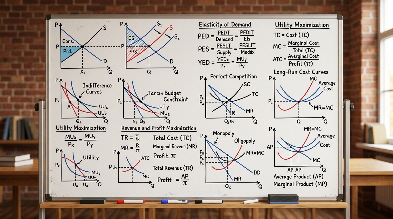
Microeconomics Formula Sheet & Key Theorems: The Complete DU Reference Guide
The ultimate cheat sheet for Intermediate Microeconomics I & II. Master Consumer Theory, Producer Theory, Market Structures, Game Theory, and Welfare Economics.
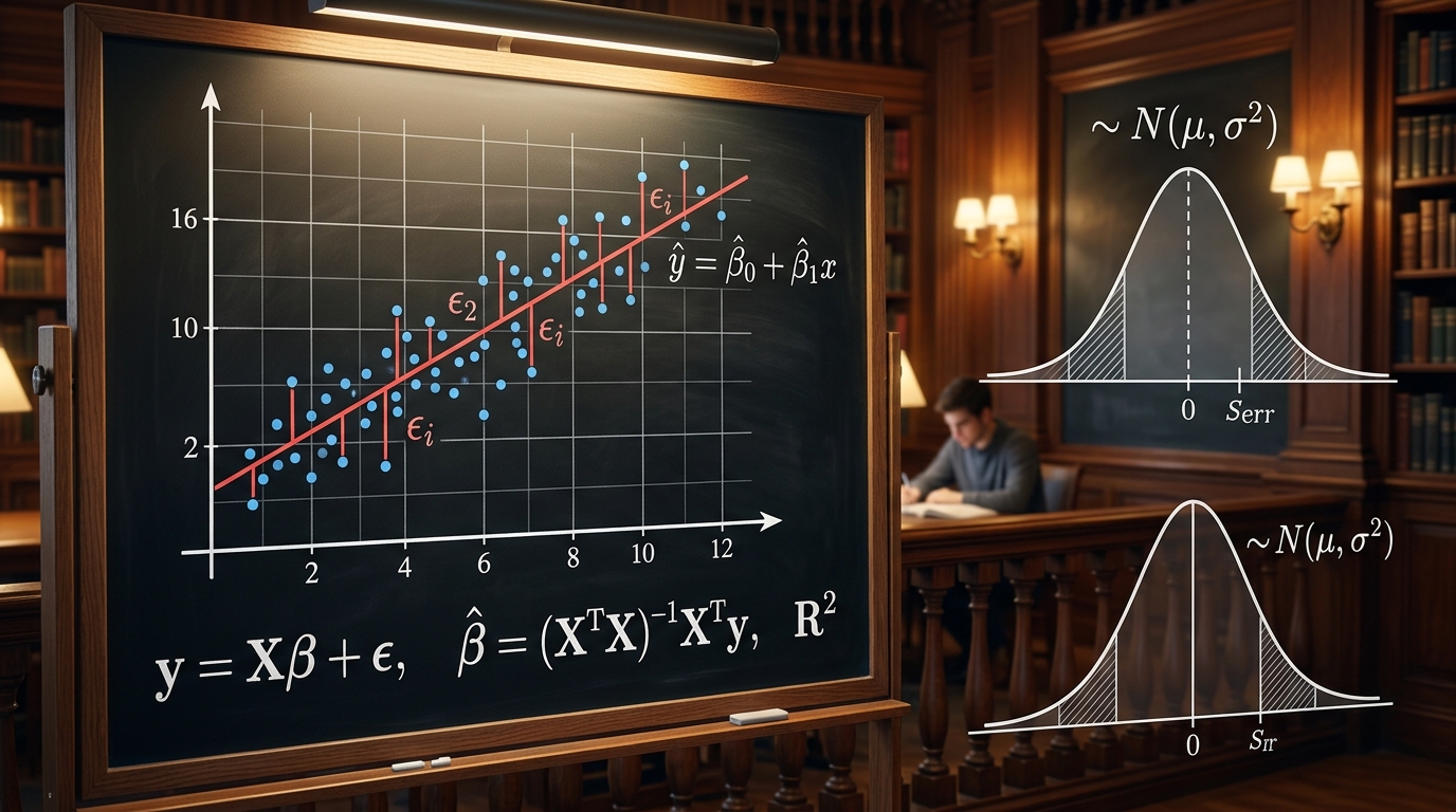
Introductory Econometrics & OLS Regression: Gauss-Markov Theorem, Proofs & Exam Numericals
Comprehensive 4,500-word masterclass on Introductory Econometrics and Ordinary Least Squares (OLS) for DU Economics students. Covers algebraic derivations of beta_0 and beta_1, Gauss-Markov BLUE proofs, R-squared variance decomposition, hypothesis testing (t and F-tests), and 3 fully worked numerical problems.
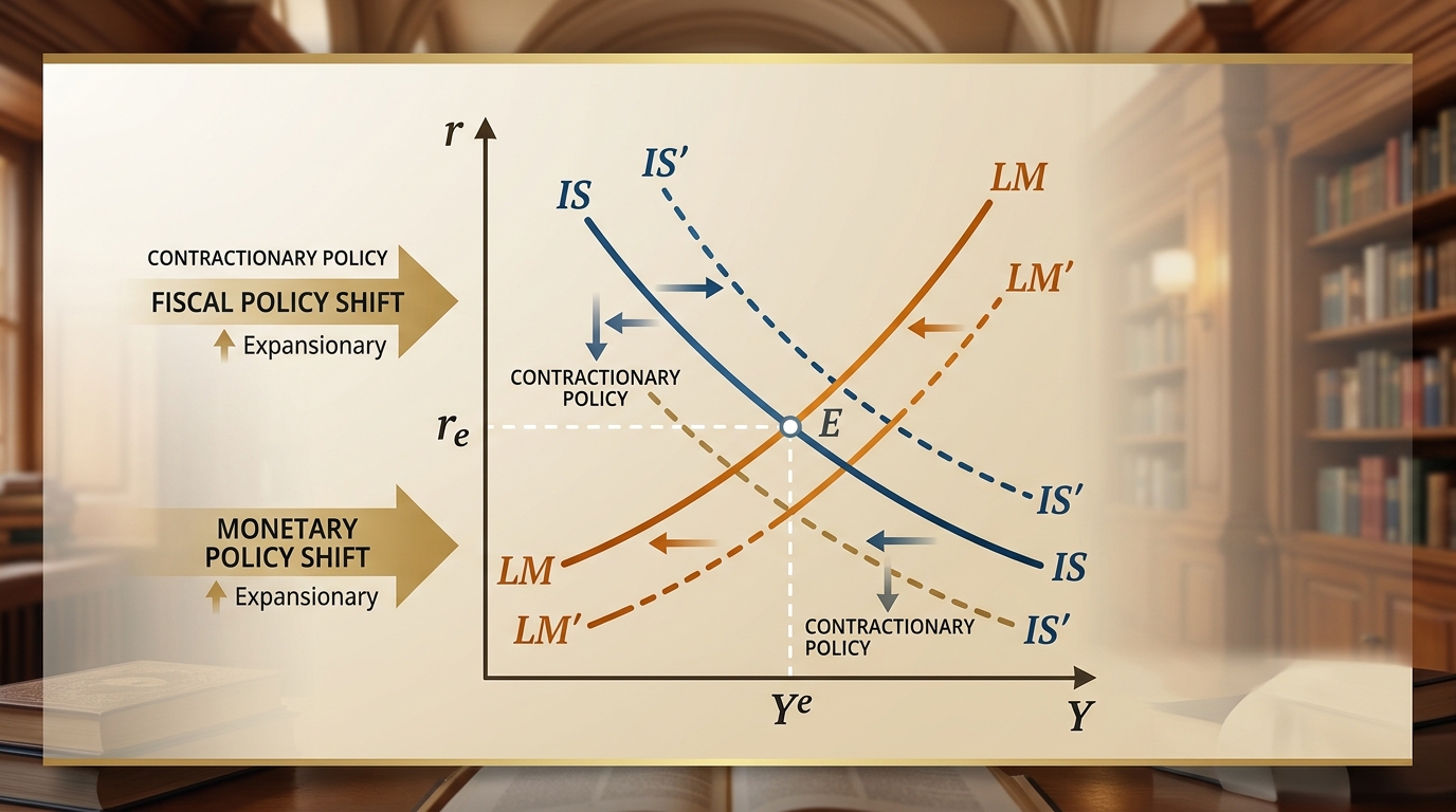
IS-LM Model: Goods & Money Market Equilibrium, Policy Multipliers & DU Exam Numericals
Comprehensive 4,000-word masterclass on the IS-LM model for DU Economics students. Covers algebraic derivations of IS and LM curves, general equilibrium, fiscal and monetary policy multipliers, crowding-out effect, liquidity trap, and 3 fully worked exam numericals.