Introductory Microeconomics Unit 4: Production Function, Isoquants & Cost Curves Notes
Detailed DU Sem 1 Unit 4 notes covering Law of Variable Proportions, Isoquants, MRTS, Returns to Scale, Euler's Theorem, Isocosts, Cost Minimization & LAC Envelope.
Welcome to Unit 4 of Delhi University's Introductory Microeconomics for Semester 1. This unit shifts our focus from the consumer's side (demand) to the producer's side (supply). We explore the technical relationship between inputs and output (Production Theory) and the economic relationship between output and costs (Cost Theory). A solid grasp of this unit is non-negotiable for understanding how firms make decisions to maximize profits or minimize costs.
1. The Production Function
A production function is a purely technical or engineering relationship between inputs (factors of production) and the maximum output that can be produced using those inputs, given the current state of technology.
Mathematically, it is expressed as: Q = f(L, K, T, E...), where Q is the total physical product (output), L is labor, K is capital, T is land (or resources), and E is entrepreneurship. For simplicity in introductory microeconomics, we assume a two-input model: Labor (L) and Capital (K). Thus, Q = f(L, K).
Total, Average, and Marginal Product
To understand production in the short run (where at least one input is fixed, typically capital K), we need to define three crucial concepts associated with the variable input (labor L).
- Total Product (TP or TPP): The total amount of output produced in a given time period by a given quantity of inputs. TP = Q = f(L, K_bar).
- Average Product (AP or APP): The total product per unit of the variable input. AP = TP / L. It represents the average productivity of labor.
- Marginal Product (MP or MPP): The addition to total product resulting from the employment of one more unit of the variable input, keeping the fixed input constant. MP = d(TP) / dL. Geometrically, MP is the slope of the TP curve.
Exact Mathematical and Geometric Relationships
The relationship between TP, AP, and MP is a favorite topic for DU examiners. You must understand the mathematical logic and the geometry of the curves.
- Relationship between TP and MP:
- As long as MP is positive, TP increases.
- When MP is increasing, TP increases at an increasing rate (convex portion of the TP curve).
- When MP reaches its maximum, the TP curve has an inflection point (changes from convex to concave).
- When MP is decreasing but still positive, TP increases at a decreasing rate.
- When MP is exactly zero, TP reaches its maximum point.
- When MP becomes negative, TP starts to decrease.
- Relationship between AP and MP:
- When MP is greater than AP (MP > AP), AP must be rising. Think of your GPA: if your new semester grade (Marginal) is higher than your cumulative GPA (Average), your cumulative GPA will rise.
- When MP is less than AP (MP < AP), AP must be falling.
- When MP equals AP (MP = AP), AP is at its maximum. Geometrically, the MP curve cuts the AP curve from above at the AP curve's peak. Also, at the maximum of AP, a ray from the origin is tangent to the TP curve.
2. Short-Run Production: The Law of Variable Proportions
The Law of Variable Proportions (also known as the Law of Diminishing Marginal Returns) is the fundamental principle of short-run production. It states that as more and more units of a variable factor (e.g., Labor) are combined with a fixed amount of other factors (e.g., Capital), the marginal product of the variable factor will eventually decline.
The Three Stages of Production
The production process in the short run is typically divided into three distinct stages based on the behavior of TP, AP, and MP.
- Stage I: Stage of Increasing Returns
- Starts from the origin (L=0) to the point where AP reaches its maximum (where AP = MP).
- In this stage, TP increases initially at an increasing rate (up to the point of inflection where MP is maximum) and then at a decreasing rate.
- MP rises, reaches a peak, and starts falling, but remains above AP. AP continues to rise throughout this stage.
- Why does this happen? The fixed factor (Capital) is abundant relative to the variable factor (Labor). Adding labor allows for better utilization of machinery and specialization of tasks.
- Stage II: Stage of Diminishing Returns (The Economic Zone)
- Starts from the point where AP is maximum (AP = MP) to the point where TP is maximum (MP = 0).
- In this stage, TP continues to increase, but strictly at a decreasing rate.
- Both AP and MP are declining, but both are positive. MP is strictly less than AP.
- Why does this happen? The ideal proportion between Labor and Capital has been passed. The fixed factor becomes increasingly scarce relative to the variable factor.
- Stage III: Stage of Negative Returns
- Starts beyond the point of maximum TP (where MP becomes negative).
- TP declines.
- AP continues to fall but remains positive. MP is negative.
- Why does this happen? The variable factor is so excessive relative to the fixed factor that workers get in each other's way, reducing total output.
Rational Economic Zone (Why Stage II?)
A rational producer will never choose to operate in Stage III because adding more workers actually reduces total output (MP < 0), which makes absolutely no economic sense. But why not Stage I? In Stage I, the marginal product of the fixed factor is technically negative. The firm is not using its fixed capital efficiently. As long as the product price is positive, a firm in a competitive market will want to expand output through Stage I because the average product of labor is still rising, meaning the cost per unit of output is falling.
Therefore, Stage II is the only relevant stage for a rational producer. In Stage II, MP and AP are falling, but both are positive. The exact level of employment within Stage II will be determined by input and output prices.
3. Long-Run Production: Isoquants and MRTS
In the long run, all factors of production are variable. The firm can scale up or scale down both Labor and Capital. We analyze long-run production using Isoquants.
What is an Isoquant?
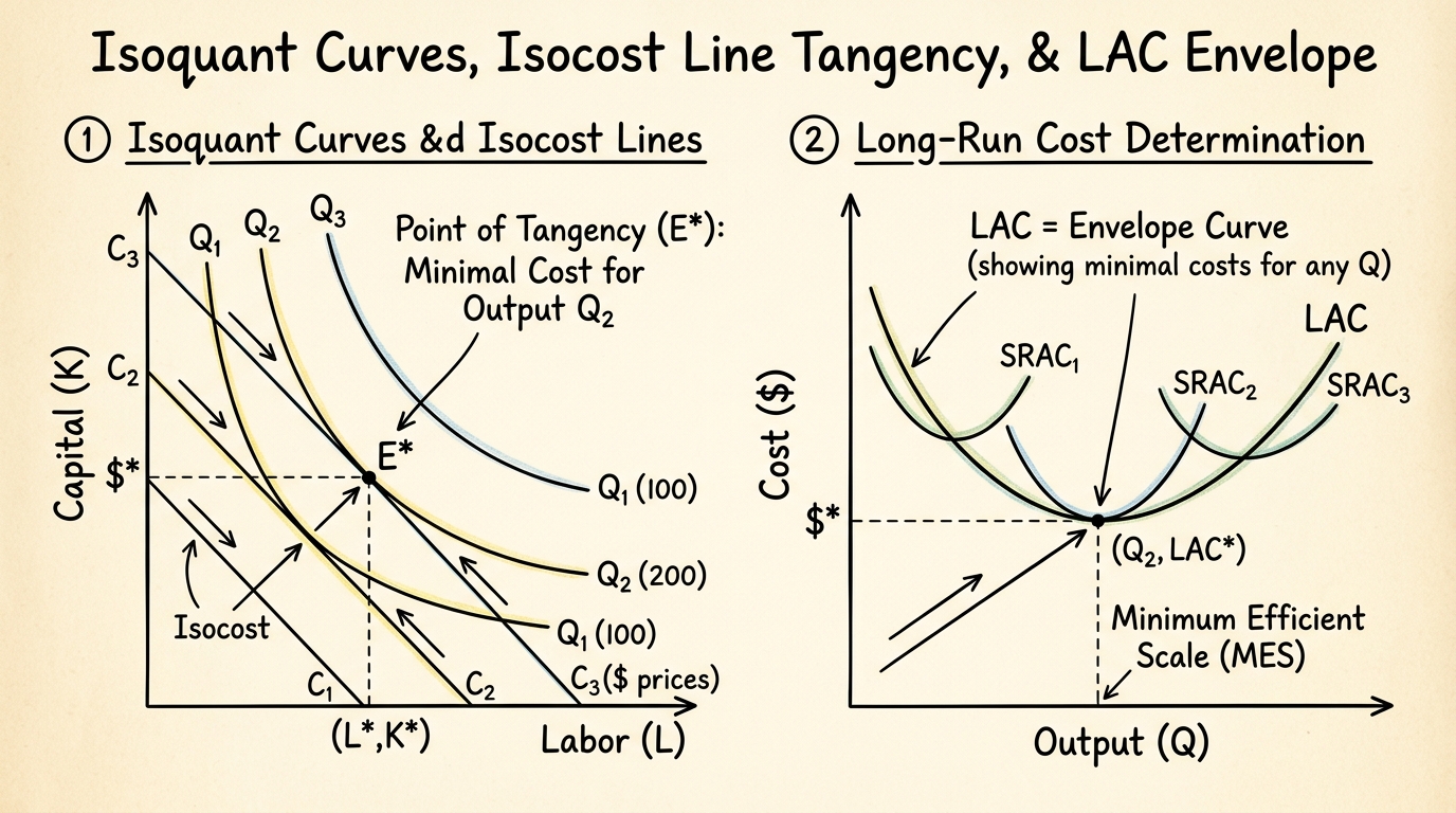
An isoquant (iso = equal, quant = quantity) is a curve representing all the different combinations of two inputs (Labor and Capital) that yield exactly the same level of total output. It is the producer's equivalent of an indifference curve.
Properties of Isoquants
- Downward Sloping (Negative Slope): If you reduce the amount of capital, you must increase the amount of labor to keep total output constant.
- Convex to the Origin: This is due to the principle of Diminishing Marginal Rate of Technical Substitution (MRTS). As you substitute more and more labor for capital, it becomes increasingly difficult to replace capital with labor.
- Higher Isoquants Mean Higher Output: An isoquant lying to the right (further from the origin) represents combinations of inputs that produce a greater total quantity.
- Isoquants Cannot Intersect: If they intersected, it would imply that a single combination of labor and capital could produce two different maximum levels of output efficiently, which violates our assumption of technical efficiency.
Marginal Rate of Technical Substitution (MRTS)
MRTS is the rate at which a firm can substitute one input for another while keeping output constant. It is the absolute value of the slope of the isoquant.
MRTS_LK = - dK / dL (The amount of capital a firm is willing to give up to get one more unit of labor).
Crucially, MRTS_LK is equal to the ratio of the marginal products of the two inputs:
Along an isoquant, the change in total output is zero. Therefore:
(MP_L * dL) + (MP_K * dK) = 0
MP_L * dL = - MP_K * dK
- dK / dL = MP_L / MP_K
MRTS_LK = MP_L / MP_K
The diminishing MRTS_LK implies that as we move down along an isoquant, MP_L falls (due to more labor) and MP_K rises (due to less capital), causing the ratio (MP_L / MP_K) to decline. This creates the convex shape.
Ridge Lines and the Economic Region of Production
While an isoquant theoretically extends indefinitely, certain parts of it represent irrational combinations. Ridge lines separate the economically relevant portions of isoquants from the irrelevant ones.
- Upper Ridge Line: Connects points on isoquants where the marginal product of capital (MP_K) is zero. Above this line, MP_K is negative (meaning MRTS is negative, isoquants slope upwards).
- Lower Ridge Line: Connects points on isoquants where the marginal product of labor (MP_L) is zero. To the right of this line, MP_L is negative.
The area bounded by the two ridge lines is the Economic Region of Production. Inside this region, the marginal products of both inputs are positive, isoquants are downward sloping, and it is rational to operate here. This is the long-run equivalent of Stage II.
4. Returns to Scale
Returns to scale describe how total output changes when all inputs are changed proportionately in the long run. If a firm doubles both labor and capital, what happens to output?
- Increasing Returns to Scale (IRS): Output increases by a greater proportion than the increase in inputs. E.g., doubling inputs triples output. This is usually due to indivisibilities, specialization, and dimensional efficiencies (like the area/volume rule in pipelines).
- Constant Returns to Scale (CRS): Output increases by exactly the same proportion as the inputs. E.g., doubling inputs exactly doubles output. This means replicating the current plant precisely.
- Decreasing Returns to Scale (DRS): Output increases by a smaller proportion than the increase in inputs. E.g., doubling inputs only increases output by 50%. This is typically caused by managerial diseconomies—communication breakdowns, bureaucracy, and coordination failures as a firm gets too large.
Cobb-Douglas Production Function and Homogeneity
The Cobb-Douglas production function is a widely used functional form: Q = A * K^alpha * L^beta.
Where A is total factor productivity, and alpha and beta are output elasticities of capital and labor, respectively.
A function is homogeneous of degree n if f(tL, tK) = t^n * f(L, K) for any t > 0. Let's test the Cobb-Douglas function by multiplying both inputs by a constant 't':
Q_new = A * (tK)^alpha * (tL)^beta
Q_new = A * (t^alpha * K^alpha) * (t^beta * L^beta)
Q_new = t^(alpha + beta) * [A * K^alpha * L^beta]
Q_new = t^(alpha + beta) * Q_initial
Thus, the Cobb-Douglas function is homogeneous of degree (alpha + beta).
- If alpha + beta = 1: Constant Returns to Scale (CRS)
- If alpha + beta > 1: Increasing Returns to Scale (IRS)
- If alpha + beta < 1: Decreasing Returns to Scale (DRS)
Euler's Product Exhaustion Theorem
Euler's Theorem states that for a production function that is homogeneous of degree 1 (CRS), if each factor of production is paid its marginal product, the total output will be exactly exhausted.
Mathematically: Q = L * MP_L + K * MP_K
Under perfect competition in input and output markets, real wage (w/P) = MP_L and real rental rate (r/P) = MP_K. Therefore, paying factors their marginal product means total wage bill plus total capital rent exactly equals total revenue (leaving zero pure economic profit). This is a fascinating result linking production theory to income distribution.
5. Isocost Lines and Cost Minimization
To find the optimal production point, we must combine technical possibilities (isoquants) with economic constraints (costs). The constraint is represented by the isocost line.
The Isocost Line
An isocost line shows all combinations of labor and capital that a firm can purchase for a given total cost, given input prices.
Equation: C = wL + rK
Where C is total cost, w is the wage rate of labor, and r is the rental rate of capital. Rearranging for K gives the equation of a line:
K = (C / r) - (w / r) * L
The vertical intercept is C/r (maximum capital if no labor is hired). The horizontal intercept is C/w. The slope of the isocost line is - w / r, the ratio of input prices.
Cost Minimization (Producer's Equilibrium)
A firm aims to produce a target level of output (a specific isoquant) at the lowest possible cost (the lowest possible isocost line).
Geometrically, this occurs at the point of tangency between the target isoquant and the lowest possible isocost line. At the point of tangency, the slopes are equal.
Slope of Isoquant (MRTS) = Slope of Isocost line
MP_L / MP_K = w / r
Rearranging this gives a powerful intuitive rule:MP_L / w = MP_K / r
This means the firm should allocate its budget such that the marginal product per rupee spent on labor equals the marginal product per rupee spent on capital. If MP_L/w > MP_K/r, the firm should shift spending from capital to labor because labor is giving more "bang for the buck" at the margin.
The Expansion Path
If we hold input prices (w and r) constant but vary the firm's budget, the isocost lines shift outwards in parallel. The firm will find new points of tangency on higher isoquants. The curve connecting all these points of tangency (cost-minimizing input combinations for every output level) is called the Expansion Path. It represents the firm's long-run total cost curve mapped in the input space. For a homogeneous production function, the expansion path is a straight line through the origin.
6. Short-Run Cost Curves
The short run implies the existence of fixed costs. Let's break down the cost family.
- Total Fixed Cost (TFC): Costs that do not vary with output (e.g., rent, insurance). The TFC curve is a horizontal line.
- Total Variable Cost (TVC): Costs that vary with output (e.g., wages, raw materials). The TVC curve starts from the origin, initially rises at a decreasing rate, and then rises at an increasing rate (due to the Law of Variable Proportions).
- Total Cost (TC): TC = TFC + TVC. The TC curve is parallel to the TVC curve, shifted vertically upwards by the amount of TFC.
Average and Marginal Costs
- Average Fixed Cost (AFC): AFC = TFC / Q. Since TFC is constant, as Q increases, AFC continuously falls. The AFC curve is a rectangular hyperbola; it approaches both axes asymptotically but never touches them. The area under the AFC curve at any point equals TFC.
- Average Variable Cost (AVC): AVC = TVC / Q. AVC typically falls, reaches a minimum, and then rises, giving it a U-shape. This U-shape is the exact mirror image of the AP curve. (When AP rises, AVC falls; when AP is maximum, AVC is minimum).
- Average Total Cost (ATC or AC): ATC = TC / Q = AFC + AVC. It is U-shaped. The minimum of ATC occurs at a higher level of output than the minimum of AVC because falling AFC pulls ATC down for a while even after AVC starts rising.
- Marginal Cost (MC): The addition to total cost from producing one more unit. MC = d(TC)/dQ = d(TVC)/dQ. The MC curve is U-shaped and mirrors the MP curve.
Crucial Geometric Relationships in Short-Run Costs
These relationships are standard 5-mark DU exam questions.
- MC cuts AVC at its minimum. (Proof: When MC < AVC, AVC falls. When MC > AVC, AVC rises. Therefore, they must be equal at the minimum of AVC).
- MC cuts ATC at its minimum. (Same logic as above).
- ATC and AVC get closer together but never touch. The vertical distance between them is AFC. Since AFC gets smaller as Q increases, the gap narrows, but since AFC never reaches zero, they never intersect.
- Relationship between Production and Cost: MC = w / MP_L and AVC = w / AP_L. This proves that cost curves are just the inverse of productivity curves. The U-shape of short-run cost curves is driven entirely by the Law of Variable Proportions.
7. Long-Run Cost Curves: The LAC Envelope
In the long run, there are no fixed costs. The firm can choose any plant size. For every possible plant size, there is a Short-Run Average Cost (SAC) curve.
The Long-Run Average Cost (LAC) Envelope Curve
The LAC curve is the locus of the cost-minimizing points for each level of output. It is derived by drawing a curve that is tangent to the lowest possible SAC curve for each output level. Because it "envelopes" all the SAC curves from below, it is called the Envelope Curve or the Planning Curve.
A key insight: The LAC curve is tangent to the minimum point of an SAC curve only at the absolute minimum of the LAC curve itself. For output levels below the LAC minimum, the LAC is tangent to the falling portion of the SAC curves. For output levels above the LAC minimum, the LAC is tangent to the rising portion of the SAC curves.
Economies and Diseconomies of Scale
The LAC curve is U-shaped (often a flatter, "saucer" shape), but not because of the Law of Variable Proportions (which requires fixed factors). The long-run U-shape is driven by Returns to Scale and Economies/Diseconomies of scale.
- Internal Economies of Scale: Causes the LAC curve to fall as output expands. Sources include technical economies (indivisibilities), managerial economies (specialization), commercial economies (bulk buying discounts), and financial economies (lower interest rates for large firms).
- Internal Diseconomies of Scale: Causes the LAC curve to rise. The primary source is managerial diseconomies—the difficulty of coordinating and controlling a massive, complex organization, leading to inefficiencies and red tape.
(Note: External economies/diseconomies shift the entire LAC curve down/up, whereas internal economies move you along the LAC curve).
8. Fully Solved Numerical Problems
Practicing numericals is critical. Here are 8 solved examples covering DU exam patterns.
Problem 1: Deriving AP and MP
Q: Given the production function Q = 6L^2 - 0.2L^3. Find the expressions for Average Product of Labor (AP_L) and Marginal Product of Labor (MP_L). Determine the level of labor where AP_L is maximized.
Solution:
1. AP_L = Q / L = (6L^2 - 0.2L^3) / L = 6L - 0.2L^2
2. MP_L = dQ / dL = d(6L^2 - 0.2L^3) / dL = 12L - 0.6L^2
3. To find where AP_L is maximized, we set its derivative to zero:
d(AP_L) / dL = 6 - 0.4L = 0 => 0.4L = 6 => L = 15 units.
Check: Alternatively, we know AP_L is max when AP_L = MP_L.
6L - 0.2L^2 = 12L - 0.6L^2
0.4L^2 - 6L = 0 => L(0.4L - 6) = 0. Ignoring L=0, we get 0.4L = 6 => L = 15. The answers match perfectly.
Problem 2: Cost Minimization
Q: A firm has the production function Q = 50 * L^0.5 * K^0.5. The price of labor (w) is 20 and the price of capital (r) is 80. The firm wishes to produce Q = 1000 units. Find the cost-minimizing combination of L and K, and the total cost.
Solution:
1. Target output: 1000 = 50 * L^0.5 * K^0.5 => 20 = L^0.5 * K^0.5 => 400 = L * K => K = 400/L (Eq. 1)
2. Tangency condition: MP_L / MP_K = w / r
MP_L = dQ/dL = 25 * L^(-0.5) * K^0.5
MP_K = dQ/dK = 25 * L^0.5 * K^(-0.5)
MRTS = MP_L / MP_K = (K^0.5 / L^0.5) / (L^0.5 / K^(-0.5)) = K / L
3. Equating MRTS to w/r: K / L = 20 / 80 = 1/4 => L = 4K (Eq. 2) (Expansion Path equation)
4. Substitute Eq. 2 into Eq. 1:
400 = (4K) * K => 4K^2 = 400 => K^2 = 100 => K = 10 units.
5. Find L: L = 4(10) = 40 units.
6. Minimum Total Cost: C = wL + rK = (20 * 40) + (80 * 10) = 800 + 800 = 1600.
Problem 3: Finding Shutdown and Break-Even Points
Q: A competitive firm has a short-run total cost curve given by TC = 100 + 10Q + 2Q^2. Find the break-even price and the shutdown price.
Solution:
1. Fixed Cost (TFC) = 100; Variable Cost (TVC) = 10Q + 2Q^2.
2. MC = d(TC)/dQ = 10 + 4Q
3. Break-Even Price: Minimum of ATC.
ATC = TC/Q = (100/Q) + 10 + 2Q.
Minimum ATC occurs where MC = ATC.
10 + 4Q = (100/Q) + 10 + 2Q => 2Q = 100/Q => 2Q^2 = 100 => Q^2 = 50 => Q = 7.07.
Break-even price (min ATC) = 10 + 4(7.07) = 38.28.
4. Shutdown Price: Minimum of AVC.
AVC = TVC/Q = 10 + 2Q.
Minimum AVC occurs where MC = AVC (or just look at the AVC equation; since Q must be positive, the min AVC is at Q=0).
10 + 4Q = 10 + 2Q => 2Q = 0 => Q = 0.
Shutdown price (min AVC at Q=0) = 10.
Problem 4: Returns to Scale Evaluation
Q: Determine the returns to scale for the following production functions: (a) Q = L^0.4 * K^0.6, (b) Q = L^2 + K^2, (c) Q = 10 * L^0.3 * K^0.5.
Solution: Test for homogeneity by scaling inputs by t.
(a) Q = L^0.4 * K^0.6. Cobb-Douglas. alpha+beta = 0.4 + 0.6 = 1. Constant Returns to Scale (CRS).
(b) f(tL, tK) = (tL)^2 + (tK)^2 = t^2 * (L^2 + K^2) = t^2 * Q. Homogeneous of degree 2. Since 2 > 1, Increasing Returns to Scale (IRS).
(c) Q = 10 * L^0.3 * K^0.5. Cobb-Douglas. alpha+beta = 0.3 + 0.5 = 0.8. Since 0.8 < 1, Decreasing Returns to Scale (DRS).
Problem 5: Marginal Rate of Technical Substitution
Q: A firm's production function is Q = min(3L, 4K). What type of production function is this, and what is its MRTS?
Solution:
This is a Leontief (fixed-proportion) production function. The inputs must be used in a fixed ratio. The isoquants are L-shaped.
Because the inputs cannot be substituted for one another to keep output constant along the efficient point (the corner of the L-shape), the Marginal Rate of Technical Substitution (MRTS) is either 0 (on the horizontal segment) or infinity (on the vertical segment), and undefined at the corner.
Problem 6: Long-Run Cost Function from Cobb-Douglas
Q: Given Q = L^0.5 * K^0.5. Input prices are w and r. Derive the long-run total cost function C(Q).
Solution:
1. Cost minimization: MRTS = w/r => K/L = w/r => L = (r/w)K.
2. Substitute into Production Function to express inputs as functions of output Q:
Q = [(r/w)K]^0.5 * K^0.5 = (r/w)^0.5 * K.
Therefore, K*(Q) = Q * (w/r)^0.5.
3. Find L*(Q): L = (r/w) * [Q * (w/r)^0.5] = Q * (r/w)^0.5.
4. Total Cost C = wL* + rK* = w[Q * (r/w)^0.5] + r[Q * (w/r)^0.5] = Q(w^0.5 * r^0.5) + Q(r^0.5 * w^0.5) = 2Q(wr)^0.5.
This shows that Long Run Total Cost is a linear function of Q, implying Constant AC and MC (which matches the CRS property of this production function).
Problem 7: Maximizing Output given a Budget Constraint
Q: A firm has a budget of Rs. 3000 to spend on Labor and Capital. The price of Labor w=50, and price of Capital r=100. The production function is Q = 10 * L * K. Find the output-maximizing quantities of L and K.
Solution:
1. Budget Constraint: 3000 = 50L + 100K.
2. Optimization condition: MP_L / MP_K = w / r
MP_L = 10K; MP_K = 10L.
MRTS = 10K / 10L = K / L.
Equating to w/r: K / L = 50 / 100 = 1/2 => L = 2K.
3. Substitute into the budget constraint:
3000 = 50(2K) + 100K => 3000 = 100K + 100K => 3000 = 200K => K = 15.
4. Find L: L = 2(15) = 30.
5. Maximum Output: Q = 10 * (30) * (15) = 4500 units.
Problem 8: Euler's Theorem Verification
Q: Verify Euler's theorem for the production function Q = A * L^0.6 * K^0.4.
Solution:
Euler's theorem states: L(dQ/dL) + K(dQ/dK) = Q (for a degree 1 homogeneous function).
1. Find MP_L (dQ/dL): 0.6 * A * L^(-0.4) * K^0.4
2. Find MP_K (dQ/dK): 0.4 * A * L^0.6 * K^(-0.6)
3. Compute L(MP_L) + K(MP_K):
L * [0.6 * A * L^(-0.4) * K^0.4] + K * [0.4 * A * L^0.6 * K^(-0.6)]
= 0.6 * A * L^0.6 * K^0.4 + 0.4 * A * L^0.6 * K^0.4
= (0.6 + 0.4) * [A * L^0.6 * K^0.4]
= 1 * Q = Q.
Theorem verified. The payments to factors exhaust the total product.
9. DU Exam Tips & 15-Mark Model Outline
Production and Costs frequently account for heavy-weightage questions in DU's final exams.
Crucial Diagram Checklist
Before you enter the exam hall, ensure you can draw these flawlessly without looking at the book:
- TP, AP, MP curves stacked: Must clearly show the inflection point aligning with max MP, and max AP intersecting MP. Label the three stages clearly.
- Isoquants and Ridge Lines: Show the convex isoquants and highlight the economic region in the middle.
- Producer's Equilibrium: Isocost line tangent to an isoquant.
- Expansion Path: Draw a few tangency points and connect them.
- Short-run Cost curves stacked: MC cutting ATC and AVC exactly at their minimum points. AFC as a rectangular hyperbola.
- LAC Envelope Curve: Draw 3-4 SAC curves and smoothly envelope them with a U-shaped LAC curve. Emphasize the tangency points correctly.
Model Answer Outline (15 Marks)
Question: "Explain the Law of Variable Proportions. Why is Stage II considered the rational zone of production?"
Outline:
- Introduction (2 marks): Define the law. State assumptions (short run, one factor fixed, homogenous variable units, constant technology).
- Table Schedule (2 marks): Create a simple hypothetical table showing L, TP, AP, and MP. Ensure the numbers reflect the three stages (increasing, diminishing, and negative returns).
- Diagram (4 marks): Draw a large, neat graph with TP on the top panel and AP, MP on the bottom panel. Clearly demarcate Stage I, II, and III. Mark the point of inflection, max AP, max TP.
- Explanation of Stages (4 marks): Briefly explain what happens to TP, AP, and MP in each stage and provide the economic intuition (e.g., better utilization of fixed factor in Stage I, over-crowding in Stage III).
- Rational Zone Justification (3 marks): Argue why Stage I is irrational (underutilization of fixed capital, MP of fixed factor is negative). Argue why Stage III is irrational (MP of labor is negative, total output falls). Conclude that Stage II (diminishing but positive returns for both factors) is the only economically rational operating region.
Mastering Unit 4 is largely about understanding the duality between production and costs. Every concept in production has a direct mirror image in costs. If you understand the MP curve, you understand the MC curve. If you grasp Isoquants, you will breeze through Isocosts and Expansion Paths. Keep practicing the numericals and sketching the graphs!
Frequently asked questions
Why does the Marginal Cost (MC) curve cut the Average Total Cost (ATC) curve at its minimum?
Mathematically, when MC is less than ATC, it pulls the average down. When MC is greater than ATC, it pulls the average up. Thus, they must intersect at the exact minimum point of ATC.
What is the difference between Returns to a Factor and Returns to Scale?
Returns to a Factor (short-run) analyzes changes in output when one factor is varied while others are fixed. Returns to Scale (long-run) analyzes changes in output when all inputs are varied proportionately.
What is Euler's Theorem in production?
Euler's Theorem states that if a production function is homogeneous of degree one (constant returns to scale) and each factor is paid its marginal product, the total output is exactly exhausted by the total factor payments.
Dhairya sat the same DU papers he now writes about. Acadly is his attempt to say the useful things his own first-year self would have wanted to hear.
Keep reading
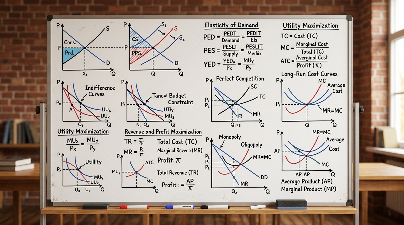
Microeconomics Formula Sheet & Key Theorems: The Complete DU Reference Guide
The ultimate cheat sheet for Intermediate Microeconomics I & II. Master Consumer Theory, Producer Theory, Market Structures, Game Theory, and Welfare Economics.
Introductory Econometrics & OLS Regression: Gauss-Markov Theorem, Proofs & Exam Numericals
Comprehensive 4,500-word masterclass on Introductory Econometrics and Ordinary Least Squares (OLS) for DU Economics students. Covers algebraic derivations of beta_0 and beta_1, Gauss-Markov BLUE proofs, R-squared variance decomposition, hypothesis testing (t and F-tests), and 3 fully worked numerical problems.
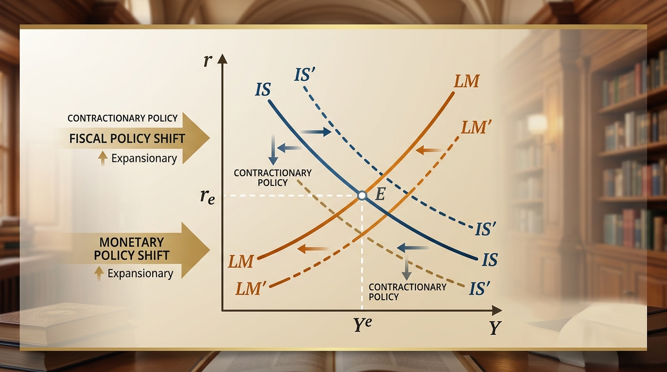
IS-LM Model: Goods & Money Market Equilibrium, Policy Multipliers & DU Exam Numericals
Comprehensive 4,000-word masterclass on the IS-LM model for DU Economics students. Covers algebraic derivations of IS and LM curves, general equilibrium, fiscal and monetary policy multipliers, crowding-out effect, liquidity trap, and 3 fully worked exam numericals.