Introductory Microeconomics Unit 3: Consumer Theory, Indifference Curves & Slutsky Notes
Complete DU Sem 1 Unit 3 notes on consumer preference axioms, utility functions (Cobb-Douglas, Leontief), budget constraint, MRS tangency, Hicksian/Slutsky decomposition & WARP.
Welcome to the most critical and conceptually demanding unit of Delhi University's Introductory Microeconomics (Semester 1) syllabus! Unit 3 is the core of Consumer Theory. This unit builds the entire framework of how consumers make choices subject to budget constraints, laying down the mathematical and graphical foundations for demand curves, price effect decompositions, and utility maximization.
If you master this unit, you have practically secured a top grade in your Microeconomics exam. The mathematical rigor introduced here will follow you into Semesters 2, 3, and beyond, especially if you pursue an Economics Honours degree. Let's dive deep into consumer preference axioms, utility functions, the budget constraint, optimal choices, the famous Slutsky equation, and the Weak Axiom of Revealed Preference (WARP).
1. The Foundation: Axioms of Consumer Preferences
Before we can mathematically model consumer behavior, we must establish a set of logical rules governing how a "rational" consumer ranks different bundles of goods. A consumption bundle, let's call it A = (X, Y), represents a specific quantity of good X and good Y.
For our theory to work flawlessly, we assume four fundamental axioms (or assumptions) about consumer preferences:
1.1 Completeness
The Completeness axiom states that given any two bundles A and B, a consumer can always compare them and make a decision. The consumer must either:
- Strictly prefer A over B (A > B)
- Strictly prefer B over A (B > A)
- Be indifferent between A and B (A ~ B)
There is no "I don't know" or "I cannot compare" option in this model. This ensures that the consumer's preference ordering covers all possible bundles in the consumption space.
1.2 Transitivity
Transitivity is the consistency axiom. It dictates that if a consumer prefers bundle A to bundle B, and bundle B to bundle C, then they MUST prefer bundle A to bundle C.
Symbolically: If A > B and B > C, then A > C.
DU Exam Tip: What happens if transitivity is violated? If A > B, B > C, but C > A, the consumer would get stuck in an infinite cycle (a "money pump" scenario) where they keep trading A for C, C for B, and B for A, paying a small fee each time until they run out of money. Transitivity guarantees that indifference curves never intersect. If they did, it would lead to illogical conclusions where A ~ B and A ~ C, but B > C, which contradicts the axiom.
1.3 Monotonicity (More is Better / Non-Satiation)
Monotonicity implies that a consumer always prefers a bundle that has more of at least one good and no less of the other. If bundle A has the same amount of Y but more of X than bundle B, then A is strictly preferred to B.
This assumption simplifies our analysis to "goods" (things you want more of) rather than "bads" (like pollution, which you want less of). Strict monotonicity ensures that indifference curves are downward sloping. If you take away some of good X, you must compensate the consumer with more of good Y to keep them on the same utility level.
1.4 Strict Convexity (Averages are preferred to extremes)
Convexity means that consumers prefer a balanced mix of goods rather than extremes. If a consumer is indifferent between bundle A (10 apples, 2 oranges) and bundle B (2 apples, 10 oranges), then any weighted average of these two bundles (like bundle C: 6 apples, 6 oranges) will be strictly preferred to the extreme bundles A and B.
Graphically, strict convexity means the indifference curve is bowed inward toward the origin. Mathematically, it implies a Diminishing Marginal Rate of Substitution (MRS), which we will explore shortly.
2. Utility Functions and Indifference Curves
Utility is simply a numerical score assigned to different consumption bundles. A utility function U(X, Y) assigns higher numbers to preferred bundles. Because utility is "ordinal" (ranking matters, not the exact magnitude), applying any strictly positive monotonic transformation (like squaring, taking the natural log, or multiplying by a positive constant) to a utility function does not change the underlying preferences or the shape of the indifference curves.
An Indifference Curve (IC) is the locus of all bundles (X, Y) that give the consumer the exact same level of utility. Let's look at the four most important types of utility functions you must know for DU exams.
2.1 Cobb-Douglas Preferences
The Cobb-Douglas utility function is the workhorse of microeconomics. It usually takes the form:
U(X, Y) = A * X^a * Y^b
Often simplified to U(X,Y) = X^a * Y^b. Here, the consumer likes both goods and views them as somewhat substitutable but not perfectly.
Characteristics:
- Indifference curves are downward sloping and strictly convex to the origin.
- They are asymptotic to the axes (meaning they never touch the X or Y axis). This implies the consumer will always choose an "interior solution" (some positive amount of both goods) as long as prices are finite.
- A very common transformation is the natural log: ln(U) = a*ln(X) + b*ln(Y). This makes derivation much easier.
2.2 Perfect Substitutes
When two goods fulfill the exact same need (e.g., Reynolds blue pen vs. Cello blue pen), they are perfect substitutes.
U(X, Y) = a*X + b*Y
Characteristics:
- Indifference curves are straight, downward-sloping lines.
- The Marginal Rate of Substitution (MRS) is constant everywhere on the curve.
- Consumers typically end up with a "corner solution," spending their entire budget on whichever good is relatively cheaper compared to its utility weight.
2.3 Perfect Complements (Leontief Preferences)
When goods must be consumed in fixed proportions (e.g., left shoes and right shoes, or 1 cup of chai with exactly 2 biscuits), they are perfect complements.
U(X, Y) = min(a*X, b*Y)
Characteristics:
- Indifference curves are L-shaped.
- The optimal consumption point is always exactly at the "kink" or vertex of the L, where a*X = b*Y.
- More of one good without the corresponding proportional increase in the other provides zero extra utility.
2.4 Quasi-Linear Preferences
These functions are linear in one good and non-linear in the other.
U(X, Y) = v(X) + Y (e.g., U(X,Y) = ln(X) + Y or U(X,Y) = X^0.5 + Y)
Characteristics:
- The indifference curves are vertically parallel. A vertical shift to a higher IC doesn't change its slope at a given X.
- There are no income effects for good X (once a threshold is reached). Any extra income is spent entirely on good Y.
3. Marginal Rate of Substitution (MRS)
The Marginal Rate of Substitution (MRS) measures the rate at which a consumer is willing to trade good Y for good X while keeping utility constant. Graphically, it is the absolute value of the slope of the indifference curve at any point.
Mathematically, MRS_xy = MUx / MUy = - dY/dX
Where MUx is the marginal utility of X (partial derivative of U with respect to X) and MUy is the marginal utility of Y (partial derivative of U with respect to Y).
3.1 Proof of Diminishing MRS
For standard strictly convex preferences (like Cobb-Douglas), the MRS decreases as we move down along the indifference curve. Why?
As you consume more and more of good X, you have an abundance of X and very little of Y. Because of the Law of Diminishing Marginal Utility, the extra satisfaction (MU) you get from one more unit of X falls, while the MU of Y (which you now have very little of) rises.
Since MRS = MUx / MUy, if the numerator (MUx) is falling and the denominator (MUy) is rising, the overall fraction (MRS) must decrease. Thus, you are willing to give up fewer and fewer units of Y to get an additional unit of X.
4. The Budget Constraint
A consumer cannot simply consume infinite amounts of goods because they are constrained by their income (M) and the market prices of the goods (Px and Py).
The budget constraint equation is: Px*X + Py*Y = M
This equation can be rearranged into a line equation (y = mx + c): Y = (M/Py) - (Px/Py)*X
Key properties of the Budget Line:
- Y-intercept: M/Py (maximum amount of Y you can buy if you spend all money on Y).
- X-intercept: M/Px (maximum amount of X you can buy if you spend all money on X).
- Slope: -Px/Py (the market rate of exchange between X and Y, or the opportunity cost of X in terms of Y).
4.1 Shifts and Rotations
If Income (M) increases while prices remain constant, the budget line shifts parallel outward. The slope (-Px/Py) does not change.
If the price of good X (Px) increases while Income and Py stay constant, the budget line pivots inward along the X-axis, becoming steeper. The Y-intercept remains exactly the same.
4.2 Real-World Application: Rationing vs Cash Transfers vs Food Stamps
Let's apply this to an Indian public policy context. Suppose the government wants to help a BPL (Below Poverty Line) family. They can give: 1. A cash transfer (e.g., PM-KISAN or basic income of ₹1000). 2. In-kind food subsidy (e.g., Free PDS rations worth ₹1000).
A cash transfer shifts the entire budget line strictly outward in a parallel fashion by the amount of the cash transfer. The consumer is free to spend this extra money on food or non-food items, leading to an interior optimum tangent to a higher indifference curve.
An in-kind transfer (like specific bags of wheat and rice) shifts the budget line outward but creates a "kink" or a horizontal segment. The consumer cannot resell the food legally, so if they wanted to consume less food than the ration amount and more non-food items, they are restricted. A cash transfer is generally preferred by classical economic theory because it maximizes utility without restricting choice, though in-kind transfers are used politically to guarantee minimum nutritional intake.
5. The Consumer Optimum (Utility Maximization)
The rational consumer wishes to reach the highest possible indifference curve while staying within their budget constraint.
5.1 Interior Solutions (Tangency Condition)
For strictly convex preferences (like Cobb-Douglas), the optimum occurs where the indifference curve is exactly tangent to the budget line.
Mathematically, at tangency, the slopes are equal: MRS_xy = Px / Py
Or equivalently: MUx / Px = MUy / Py. This translates to the "equi-marginal principle" — the marginal utility per rupee spent on good X must equal the marginal utility per rupee spent on good Y.
To solve these problems algebraically, you can also use the Lagrange Multiplier Method: L = U(X, Y) + Lambda * (M - Px*X - Py*Y)
Taking partial derivatives with respect to X, Y, and Lambda, and setting them to zero will yield the demand functions X* and Y*.
5.2 Corner Solutions
A corner solution occurs when the highest utility is achieved by spending all income on just one good. This typically happens with Perfect Substitutes or when preferences are concave.
For Perfect Substitutes U = aX + bY, the MRS is constant at a/b.
- If MRS > Px/Py, the consumer only buys X. X* = M/Px, Y* = 0.
- If MRS < Px/Py, the consumer only buys Y. X* = 0, Y* = M/Py.
- If MRS = Px/Py, any bundle on the budget line gives the exact same utility.
6. Income and Price Consumption Curves
6.1 Income Consumption Curve (ICC) & Engel Curves
As income (M) increases, the budget line shifts outward. The Income Consumption Curve (ICC) is the locus of all optimal consumer bundles at different levels of income, holding prices constant.
From the ICC, we can plot the Engel Curve, which graphs the relationship between Income (on Y-axis) and the quantity demanded of a specific good (on X-axis).
- For Normal Goods: The Engel curve is upward sloping.
- For Inferior Goods: The Engel curve bends backward; as income rises beyond a point, demand falls.
6.2 Price Consumption Curve (PCC) & Demand Curve Derivation
If we hold income and the price of Y constant, but lower the price of X, the budget line pivots outward along the X-axis. The locus of new tangency points forms the Price Consumption Curve (PCC).
Mapping the price of X against the optimal quantity of X derived from the PCC gives us the Individual Demand Curve! Because it is derived from tangency points where utility is maximized subject to a budget constraint, the standard uncompensated demand curve is known as the Marshallian Demand Curve.
7. Slutsky vs Hicksian Price Effect Decomposition
When the price of a good falls, you buy more of it for two distinct reasons. This is the most frequently tested essay topic in DU Microeconomics!
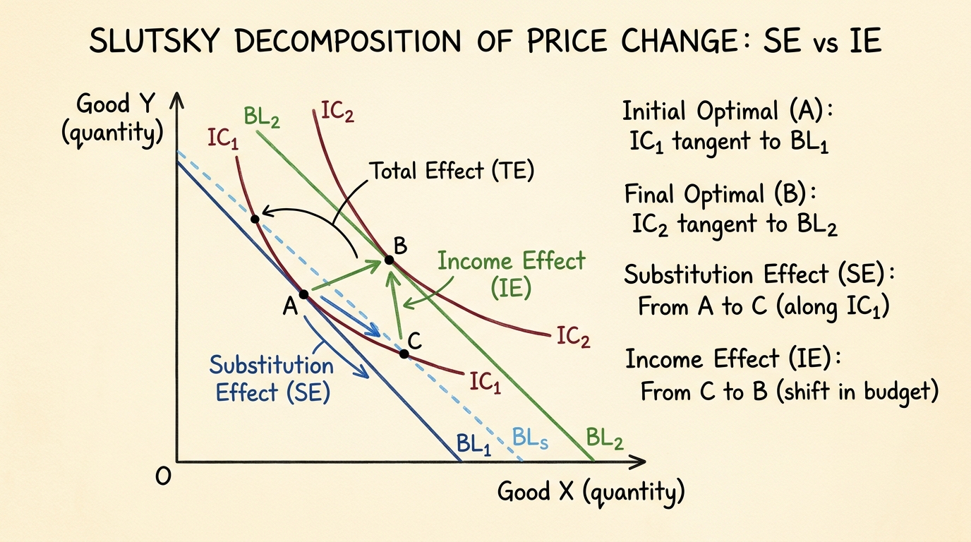
Total Price Effect (TE) = Substitution Effect (SE) + Income Effect (IE)
7.1 The Substitution Effect (SE)
When good X becomes relatively cheaper than Y, consumers naturally substitute away from Y towards X. The Substitution Effect is ALWAYS negative (meaning price and quantity move in opposite directions). If price falls, SE causes quantity to rise.
7.2 The Income Effect (IE)
When the price of good X falls, your purchasing power (real income) effectively increases. You feel richer. How you spend this extra "real income" depends on the nature of the good.
- Normal Goods: A rise in real income leads to a rise in demand. The IE reinforces the SE. (TE is large).
- Inferior Goods: A rise in real income leads to a fall in demand. The IE opposes the SE, but the SE is usually stronger. The demand curve is still downward sloping, but steeper.
- Giffen Goods: An extreme inferior good where the negative IE is so powerful it completely overpowers the SE. A price drop leads to an overall drop in quantity demanded. The demand curve is upward sloping! Example: very poor households consuming cheap staple foods.
7.3 Hicksian vs. Slutsky Approaches
To isolate the SE from the IE, we must imagine taking away just enough income from the consumer so they don't feel the "income effect" of the price drop. How we define this "constant real income" differs between Hicks and Slutsky.
Hicksian Decomposition
John Hicks defined constant real income as keeping utility constant. After the price drops, we mathematically draw a hypothetical budget line parallel to the new prices, but tangent to the original indifference curve. The movement along the original IC is the pure Hicksian Substitution Effect.
Slutsky Decomposition
Eugen Slutsky defined constant real income as keeping purchasing power constant, meaning the consumer must just be able to afford their original bundle of goods. We draw a hypothetical budget line parallel to the new prices that passes exactly through the original consumption bundle. The consumer will usually move to a higher IC on this hypothetical budget line. The movement from the old bundle to the new bundle on this pivot line is the Slutsky Substitution Effect.
Slutsky Equation: dX/dPx = (dX/dPx)_compensated - X * (dX/dM)
8. Revealed Preference Theory (WARP)
What if we cannot observe a consumer's abstract indifference curves or utility function? Paul Samuelson argued we only need to observe their actual purchasing behavior in the market. If a consumer chooses bundle A when bundle B is also affordable, A is "directly revealed preferred" to B.
The Weak Axiom of Revealed Preference (WARP)
WARP states: If bundle A is directly revealed preferred to bundle B, then bundle B can NEVER be directly revealed preferred to bundle A in any other price situation.
If the consumer bought A when B was cheaper or equally priced, it means they genuinely like A better. If tomorrow prices change and both A and B are affordable, they must not suddenly choose B over A. If they do, they violate WARP and are acting irrationally.
Mathematically, if P1*A >= P1*B (A chosen over affordable B at prices P1), then it must NOT be true that P2*B >= P2*A (B chosen over affordable A at prices P2).
9. 8 Fully Solved Numericals for DU Exams
Problem 1: Cobb-Douglas Utility Maximization
Q: A consumer has utility U = X^0.5 * Y^0.5. Income M = 100, Px = 2, Py = 5. Find optimal bundle.
Step 1: Find MUx and MUy.
MUx = 0.5 * X^-0.5 * Y^0.5
MUy = 0.5 * X^0.5 * Y^-0.5
Step 2: Set MRS = Px/Py.
MRS = MUx / MUy = Y / X
Y / X = 2 / 5 => Y = (2/5)X
Step 3: Substitute into Budget Constraint.
2X + 5Y = 100
2X + 5((2/5)X) = 100
2X + 2X = 100 => 4X = 100 => X* = 25.
Y* = (2/5)*25 = 10.
Answer: Bundle is (25, 10).
Problem 2: Perfect Substitutes Corner Solution
Q: U = 3X + Y. M = 120, Px = 4, Py = 2. Find optimal bundle.
Solution:
MRS = MUx / MUy = 3 / 1 = 3.
Price ratio Px/Py = 4 / 2 = 2.
Since MRS (3) > Px/Py (2), the consumer gets more bang for their buck from X. They will spend all money on X.
X* = 120 / 4 = 30. Y* = 0.
Answer: (30, 0).
Problem 3: Leontief Perfect Complements
Q: U = min(2X, Y). M = 100, Px = 2, Py = 4.
Solution:
Optimal choice always satisfies 2X = Y.
Substitute Y = 2X into budget constraint:
2X + 4(2X) = 100
2X + 8X = 100 => 10X = 100 => X* = 10.
Y* = 2(10) = 20.
Answer: (10, 20).
Problem 4: Slutsky Decomposition Calculation
Q: U = X*Y. Initial M = 120, Px = 4, Py = 2. Then Px drops to 2. Find SE, IE, and TE using Slutsky method.
Step 1: Original Optimal Bundle (Bundle A).
MRS = Y/X = 4/2 = 2 => Y = 2X.
4X + 2(2X) = 120 => 8X = 120 => X1 = 15, Y1 = 30.
Step 2: New Final Bundle (Bundle C).
New prices: Px = 2, Py = 2.
MRS = Y/X = 2/2 = 1 => Y = X.
2X + 2(X) = 120 => 4X = 120 => X2 = 30, Y2 = 30.
Total Effect (TE) on X = 30 - 15 = +15 units.
Step 3: Slutsky Compensated Income (M').
How much money is needed to buy original bundle (15, 30) at NEW prices (Px=2, Py=2)?
M' = Px'*X1 + Py'*Y1 = 2(15) + 2(30) = 30 + 60 = 90.
Step 4: Intermediate Bundle (Bundle B).
Maximize U=XY subject to M'=90 and new prices Px=2, Py=2.
Y = X.
2X + 2X = 90 => 4X = 90 => X_inter = 22.5.
Step 5: Decompose.
Substitution Effect (SE) = X_inter - X1 = 22.5 - 15 = +7.5.
Income Effect (IE) = X2 - X_inter = 30 - 22.5 = +7.5.
TE = SE + IE = 7.5 + 7.5 = 15.
Problem 5: Quasi-Linear Preferences
Q: U = 2 * X^0.5 + Y. Px = 1, Py = 2, M = 10.
Solution:
MUx = X^-0.5. MUy = 1.
MRS = X^-0.5 / 1 = X^-0.5.
Set MRS = Px/Py = 1/2.
1 / X^0.5 = 1/2 => X^0.5 = 2 => X* = 4.
Substitute into budget: 1(4) + 2(Y) = 10 => 2Y = 6 => Y* = 3.
Answer: (4, 3). Note how demand for X does not depend on M (no income effect for X).
Problem 6: WARP Violation Check
Q: At P1 = (2, 2), consumer buys A=(10, 5). At P2 = (1, 3), consumer buys B=(6, 8). Is WARP violated?
Step 1: Cost of B at P1 prices.
P1*B = 2(6) + 2(8) = 12 + 16 = 28.
Cost of A at P1 prices = 2(10) + 2(5) = 30.
Since 30 > 28, the consumer could have afforded B when they chose A. Therefore, A is directly revealed preferred to B.
Step 2: Cost of A at P2 prices.
P2*A = 1(10) + 3(5) = 10 + 15 = 25.
Cost of B at P2 prices = 1(6) + 3(8) = 6 + 24 = 30.
Since 30 > 25, the consumer could have afforded A when they chose B. Therefore, B is directly revealed preferred to A.
Conclusion: WARP is heavily violated. The consumer is inconsistent.
Problem 7: Composite Good Convention
Q: Treat Y as a composite good (all other goods) with Py = 1. If U = X^2 * Y^3, find the demand curve for X.
Solution:
MRS = (2X*Y^3) / (X^2*3Y^2) = 2Y / 3X.
Set MRS = Px / 1.
2Y / 3X = Px => Y = 1.5 * Px * X.
Budget constraint: Px*X + 1*Y = M.
Px*X + 1.5*Px*X = M
2.5*Px*X = M
X* = M / (2.5 * Px) = 0.4 * M / Px.
This is the Marshallian demand curve for X.
Problem 8: Rationing Constraints
Q: U = XY. Px=2, Py=2, M=40. Government rations X to a maximum of 5 units. Find the new optimum bundle.
Solution:
Without rationing: MRS = Y/X = Px/Py = 1 => Y=X.
2X + 2X = 40 => 4X = 40 => X=10, Y=10.
With rationing (X <= 5): The consumer wants 10 units of X but can only buy 5. They are forced to stop at X=5.
If X=5, they spend 2*5 = 10 rupees. They have 30 rupees left.
They spend the remaining 30 on Y. Y = 30/2 = 15.
Answer: The new constrained optimum is (5, 15). Utility drops from 100 to 75.
10. DU PYQ Focus & Exam Writing Blueprint
In Delhi University exams, you cannot just write math. You need to structure your answers logically.
- Graph First: Almost every 10-marker or 15-marker requires a well-labeled graph. Put quantity of X on the horizontal axis and Y on the vertical axis. Clearly label the budget line shifts, tangency points, and any specific points (like Hicksian compensated points).
- Define Terms: Never use abbreviations like MRS or IC without defining them first. E.g., "The Marginal Rate of Substitution is defined as..."
- Write the Math Step-by-Step: The examiner will look for your first-order conditions. Always write out the Lagrange function or the MRS = Px/Py condition explicitly before solving.
- Conclusion: For theoretical questions (like comparing Slutsky and Hicks), write a concluding paragraph summarizing which method gives a larger substitution effect in the real world (Slutsky's compensation usually leaves the consumer slightly better off, hence the Slutsky SE is slightly larger or equal to the Hicksian SE).
By mastering these concepts, derivations, and numerical types, you are fully prepared for Unit 3 of your DU Microeconomics exam. Keep practicing the calculus, draw the graphs repeatedly until they are muscle memory, and remember: rationality in economics just means consistency in choices!
Frequently asked questions
What is the difference between Slutsky and Hicksian decompositions?
Hicks holds utility constant, keeping the consumer on the original indifference curve. Slutsky holds purchasing power constant, allowing the consumer to buy their exact original bundle at new prices.
When do corner solutions occur in consumer theory?
Corner solutions typically occur with perfect substitutes, where the consumer spends their entire budget on one good because the MRS does not equal the price ratio.
What does the Weak Axiom of Revealed Preference (WARP) state?
If bundle A is chosen over an affordable bundle B in one situation, bundle B can never be chosen over bundle A when both are affordable in a different situation.
Dhairya sat the same DU papers he now writes about. Acadly is his attempt to say the useful things his own first-year self would have wanted to hear.
Keep reading
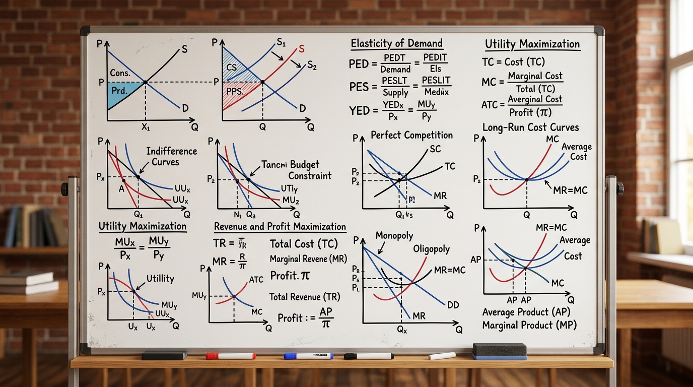
Microeconomics Formula Sheet & Key Theorems: The Complete DU Reference Guide
The ultimate cheat sheet for Intermediate Microeconomics I & II. Master Consumer Theory, Producer Theory, Market Structures, Game Theory, and Welfare Economics.

Introductory Econometrics & OLS Regression: Gauss-Markov Theorem, Proofs & Exam Numericals
Comprehensive 4,500-word masterclass on Introductory Econometrics and Ordinary Least Squares (OLS) for DU Economics students. Covers algebraic derivations of beta_0 and beta_1, Gauss-Markov BLUE proofs, R-squared variance decomposition, hypothesis testing (t and F-tests), and 3 fully worked numerical problems.
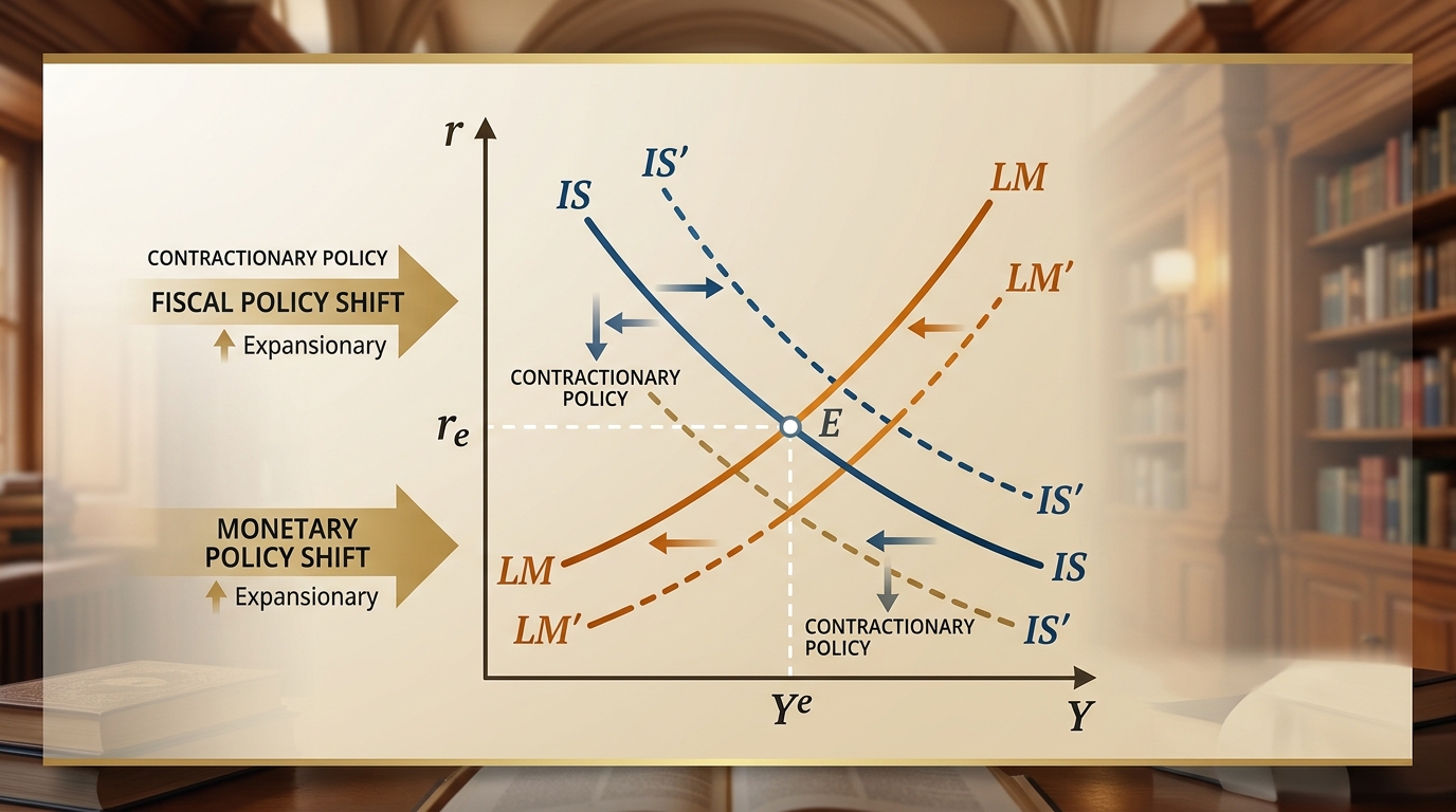
IS-LM Model: Goods & Money Market Equilibrium, Policy Multipliers & DU Exam Numericals
Comprehensive 4,000-word masterclass on the IS-LM model for DU Economics students. Covers algebraic derivations of IS and LM curves, general equilibrium, fiscal and monetary policy multipliers, crowding-out effect, liquidity trap, and 3 fully worked exam numericals.