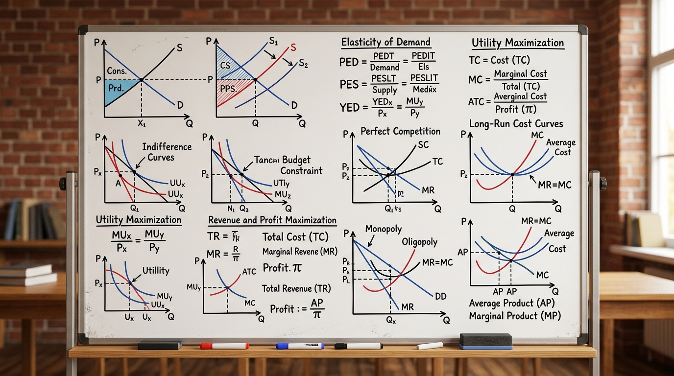
Introductory Microeconomics Unit 2: Demand, Supply, Elasticity & Market Equilibrium Notes

Introduction to Unit 2: The Core of Microeconomics

Welcome to the most fundamental unit of your Introductory Microeconomics syllabus at Delhi University: Unit 2 covering Demand, Supply, Elasticity, and Market Equilibrium. If Unit 1 was about the overarching principles of economics, Unit 2 provides the actual tools that economists use every single day to analyze how markets function.

In this comprehensive 3,000+ word study guide, we are going to dive deep into how consumers decide what to buy (demand), how producers decide what to sell (supply), how they come together (market equilibrium), how responsive they are to changes (elasticity), and what happens when the government steps in (price controls and taxes). This unit is heavily numerical and analytical. Mastering it is non-negotiable for passing Sem 1 Microeconomics, as a significant portion of your final exam—especially the 10-15 mark numerical and analytical questions—will come straight from these concepts. Let's get started.

1. The Theory of Demand

Individual vs. Market Demand

Demand is defined as the quantity of a good or service that consumers are willing and able to purchase at various possible prices during a specified period of time, ceteris paribus (other things being equal). It is crucial to understand that demand implies both the desire for a product and the financial backing to pay for it.

Individual Demand refers to the quantity demanded by a single consumer at different prices.
Market Demand is the horizontal summation of all individual demand curves in the market. If Consumer A demands 5 units at Price Rs. 10 and Consumer B demands 7 units at the same price, the market demand at Rs. 10 is 12 units.

The Law of Demand

The Law of Demand states that, ceteris paribus, there is an inverse relationship between the price of a good and its quantity demanded. When price rises, quantity demanded falls, and when price falls, quantity demanded rises. The rationale behind the downward-sloping demand curve comes from two main effects:

• Substitution Effect: As the price of a good falls, it becomes relatively cheaper compared to its substitutes, leading consumers to switch towards it.
• Income Effect: As the price falls, the consumer's real income (purchasing power) increases, allowing them to buy more of the good.

Determinants of Demand

While price determines the quantity demanded along a given curve, several other factors determine the position of the demand curve itself:

1. Income of the Consumer: For normal goods, demand increases as income rises. For inferior goods, demand falls as income rises.
2. Prices of Related Goods:
   • Substitutes: E.g., Tea and Coffee. An increase in the price of tea leads to an increase in the demand for coffee.
   • Complements: E.g., Cars and Petrol. An increase in the price of cars leads to a decrease in the demand for petrol.
3. Tastes and Preferences: Favorable changes increase demand; unfavorable changes decrease it.
4. Expectations: If consumers expect future prices to rise, current demand increases.
5. Number of Buyers: An increase in population or market size increases market demand.

Movements vs. Shifts in Demand

A common pitfall in DU exams is confusing these two concepts.

• Movement along the demand curve (Change in Quantity Demanded): Caused ONLY by a change in the price of the good itself. An upward movement is a contraction of demand; a downward movement is an expansion of demand.
• Shift of the demand curve (Change in Demand): Caused by a change in any factor other than the good's own price (e.g., income, tastes). A rightward shift is an increase in demand; a leftward shift is a decrease in demand.

Exceptions to the Law of Demand

Normally, demand curves slope downwards. However, there are two famous exceptions where the curve may slope upwards (positive relationship between price and quantity):

• Giffen Goods: Strongly inferior goods where the negative income effect dominates the substitution effect. E.g., cheap staple foods during a famine. As price rises, consumers are so impoverished that they must buy more of the staple and less of expensive foods like meat.
• Veblen Goods: Goods of ostentation or status symbols (e.g., diamonds, designer bags). The higher the price, the greater the snob appeal, and therefore the higher the quantity demanded.

2. The Theory of Supply

Supply is the quantity of a good that producers are willing and able to offer for sale at various prices during a specific period. The Law of Supply states that, ceteris paribus, there is a direct (positive) relationship between price and quantity supplied. Producers want to maximize profit; higher prices offer higher profit margins, incentivizing more production.

Determinants of Supply

1. Input Prices (Cost of Production): If wages or raw material prices rise, the cost of production increases, reducing profitability and decreasing supply (leftward shift).
2. Technology: Technological advancements lower production costs, increasing supply (rightward shift).
3. Prices of Related Goods in Production: If a farmer can grow either wheat or corn, an increase in the price of wheat will lead the farmer to substitute land away from corn towards wheat, decreasing the supply of corn.
4. Number of Sellers: More firms entering the market increases market supply.
5. Government Policy: Taxes on production decrease supply; subsidies increase supply.

Movements vs. Shifts in Supply

• Movement (Change in Quantity Supplied): Caused by a change in the good's own price. Expansion (upward movement) or Contraction (downward movement).
• Shift (Change in Supply): Caused by non-price factors. Increase (rightward shift) or Decrease (leftward shift).

3. Market Equilibrium

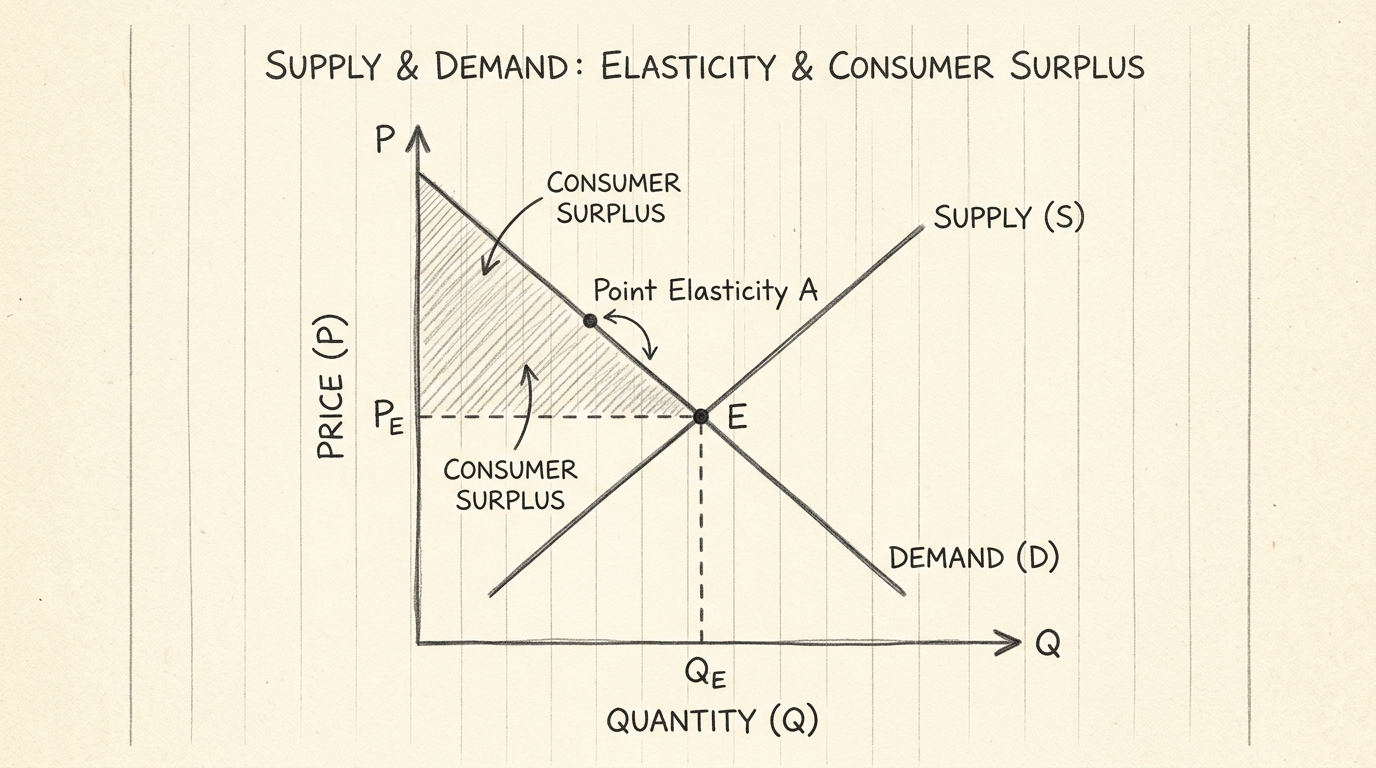
Market equilibrium occurs at the price where Quantity Demanded (Qd) equals Quantity Supplied (Qs). Graphically, this is the intersection of the downward-sloping demand curve and the upward-sloping supply curve. The price at this intersection is the equilibrium price (Pe), and the quantity is the equilibrium quantity (Qe).

Excess Demand and Excess Supply

• Excess Supply (Surplus): Occurs when the current market price is above the equilibrium price (Qs > Qd). Producers compete by lowering the price to clear inventory. As price falls, Qd expands and Qs contracts until equilibrium is restored.
• Excess Demand (Shortage): Occurs when the current market price is below the equilibrium price (Qd > Qs). Consumers compete for the limited goods, driving the price up. As price rises, Qs expands and Qd contracts until equilibrium is restored.

Stability of Equilibrium: Walrasian vs. Marshallian

In DU exams, they sometimes ask to differentiate between the two adjustment mechanisms:

• Walrasian Stability: Focuses on price adjustment. If Qd differs from Qs, price will adjust. If there's excess demand, price rises; if excess supply, price falls. The equilibrium is Walrasian stable if these price changes push the market back to Pe.
• Marshallian Stability: Focuses on quantity adjustment. Producers look at the Demand Price (what consumers are willing to pay) and Supply Price (what producers require to supply). If Demand Price > Supply Price, producers increase quantity. If Demand Price < Supply Price, producers decrease quantity. The market is Marshallian stable if these quantity adjustments push the market back to Qe.

4. Elasticity of Demand

Elasticity measures the responsiveness of one variable to changes in another. It's not enough to know that demand falls when price rises; we need to know by how much.

Price Elasticity of Demand (PED)

PED measures the percentage change in quantity demanded resulting from a 1% change in price.
Formula: PED = (Percentage change in Qd) / (Percentage change in P)
Symbolically: PED = (dQ/dP) * (P/Q)

Because of the inverse relationship (Law of Demand), PED is technically negative, but we often take the absolute value |e| for interpretation.

• Perfectly Inelastic (|e| = 0): Quantity doesn't change at all (vertical curve). E.g., lifesaving drugs.
• Inelastic (|e| < 1): Quantity changes by a smaller percentage than price. E.g., salt, basic food.
• Unit Elastic (|e| = 1): Quantity changes by the exact same percentage as price. (A rectangular hyperbola demand curve).
• Elastic (|e| > 1): Quantity changes by a larger percentage than price. E.g., luxury goods, foreign holidays.
• Perfectly Elastic (|e| = infinity): Any price increase drops demand to zero (horizontal curve). E.g., firm demand in perfect competition.

Methods of Measuring PED

1. Point Elasticity: Used for very small changes in price along a continuous demand curve. PED = (dQ/dP) * (P/Q). Geometrically on a linear demand curve, Point Elasticity = Lower Segment / Upper Segment.
2. Arc / Midpoint Method: Used for larger price changes between two points. It uses average price and average quantity to avoid the base-point problem.
   Arc PED = [(Q2 - Q1) / ((Q2 + Q1)/2)] / [(P2 - P1) / ((P2 + P1)/2)]
3. Total Outlay / Total Expenditure Method: Total Expenditure (TE) = Price * Quantity.
   • If P falls and TE rises -> Elastic (|e| > 1).
   • If P falls and TE falls -> Inelastic (|e| < 1).
   • If P falls and TE is unchanged -> Unitary (|e| = 1).

Linear Demand Curve Elasticity Proof

A frequent 5-mark proof in exams is showing that elasticity varies along a downward-sloping linear demand curve: Q = a - bP.
Since slope (dQ/dP) is constant at -b.
PED = (dQ/dP) * (P/Q) = -b * (P/Q).
At the price axis intercept (where Q = 0), P/Q approaches infinity, so |e| = infinity.
At the quantity axis intercept (where P = 0), P/Q = 0, so |e| = 0.
At the exact midpoint of the curve, |e| = 1. The upper half is elastic (>1) and the lower half is inelastic (<1).

Income Elasticity of Demand (YED)

YED measures responsiveness of demand to changes in consumer income.
Formula: YED = (Percentage change in Qd) / (Percentage change in Income)
This is used to classify goods using Engel curves:

• YED > 0 (Positive): Normal Good. If 0 < YED < 1, it's a Necessity. If YED > 1, it's a Luxury.
• YED < 0 (Negative): Inferior Good.
• YED = 0: Income neutral (e.g., salt).

Cross-Price Elasticity of Demand (XED)

XED measures how the quantity demanded of Good X responds to a change in the price of Good Y.
Formula: XED = (Percentage change in Qd of X) / (Percentage change in P of Y)

• XED > 0: Goods are Substitutes (e.g., Coke and Pepsi). Price of Y rises, demand for X rises.
• XED < 0: Goods are Complements (e.g., Cars and Petrol). Price of Y rises, demand for X falls.
• XED = 0: Goods are Unrelated.

5. Price Elasticity of Supply (PES)

PES measures how much the quantity supplied responds to changes in price.
Formula: PES = (Percentage change in Qs) / (Percentage change in P)
Because supply curves slope upwards, PES is typically positive.

Time Horizons in PES

The most important determinant of PES is time. How quickly can producers adjust their inputs to produce more?

• Momentary Period (Market Period): Supply is fixed. Firms cannot change production instantly. Supply is perfectly inelastic (vertical curve). PES = 0.
• Short Run: Firms can change variable inputs (like labor) but not fixed inputs (like factory size). Supply is somewhat elastic. PES > 0 but relatively low.
• Long Run: All inputs are variable. Firms can build new factories, and new firms can enter the market. Supply is highly elastic. PES is large.

6. Government Intervention & Welfare Analysis

Free markets reach equilibrium on their own, but governments often intervene if they believe the equilibrium price is "unfair" to buyers or sellers.

Price Ceilings

A legal maximum price set below the market equilibrium. The goal is to protect consumers (e.g., Rent Control in Delhi).
Effects: Because the price cannot rise to clear the market, a permanent shortage (Excess Demand) is created. Qd > Qs.
Consequences: Black markets emerge where goods are sold illegally at higher prices. Non-price rationing mechanisms like long queues or favoritism are used to allocate the scarce goods. Quality often deteriorates.

Price Floors

A legal minimum price set above the market equilibrium. The goal is to protect producers (e.g., Minimum Support Price or MSP for farmers in India, Minimum Wage laws).
Effects: Because the price cannot fall to clear the market, a permanent surplus (Excess Supply) is created. Qs > Qd.
Consequences: In the case of MSP, the government usually has to buy up the surplus grain to maintain the floor price, leading to massive storage costs (e.g., FCI godowns). In the labor market, a minimum wage above equilibrium creates unemployment.

Taxes, Tax Incidence, and Deadweight Loss

When the government imposes a specific (per-unit) tax on a good, it drives a wedge between the price buyers pay (Pb) and the price sellers receive (Ps). Tax = Pb - Ps.
Tax Incidence (Who bears the burden?): The burden of a tax does NOT depend on whom the government legally levies the tax. It depends entirely on relative elasticities.

• Rule: The less elastic (more rigid) side of the market bears the larger share of the tax burden.
• If Demand is more inelastic than Supply, Consumers bear most of the tax.
• If Supply is more inelastic than Demand, Producers bear most of the tax.

Deadweight Loss (DWL): Also known as excess burden. It is the loss in total surplus (consumer surplus + producer surplus) that occurs because the tax reduces the equilibrium quantity below the socially optimal free-market level. The tax prevents some mutually beneficial trades from taking place.

7. Solved Numerical Problems

Numericals are the bread and butter of the Microeconomics Sem 1 exam. You must practice them extensively. Here are 8 fully solved varieties.

Problem 1: Finding Equilibrium

Q: Given Demand: Qd = 500 - 10P and Supply: Qs = 100 + 10P. Find the equilibrium price and quantity.
Solution:
At equilibrium, Qd = Qs.
500 - 10P = 100 + 10P
400 = 20P
P = 20
Substitute P back into either equation to find Q:
Q = 500 - 10(20) = 500 - 200 = 300.
Equilibrium Price = Rs. 20, Equilibrium Quantity = 300 units.

Problem 2: Point Elasticity of Demand

Q: For the demand function Qd = 100 - 2P, calculate the price elasticity of demand at P = 25.
Solution:
First, find Q at P = 25: Qd = 100 - 2(25) = 100 - 50 = 50.
Formula for point elasticity: e = (dQ/dP) * (P/Q)
The slope dQ/dP is the coefficient of P, which is -2.
e = (-2) * (25 / 50) = -2 * 0.5 = -1.
The elasticity is -1 (Unit Elastic).

Problem 3: Arc Elasticity

Q: When the price of a good increases from Rs. 10 to Rs. 12, the quantity demanded falls from 100 to 80 units. Calculate the Arc Price Elasticity.
Solution:
P1 = 10, P2 = 12. Q1 = 100, Q2 = 80.
Change in Q = 80 - 100 = -20. Average Q = (100 + 80)/2 = 90.
Change in P = 12 - 10 = 2. Average P = (10 + 12)/2 = 11.
Arc Elasticity = (Change in Q / Average Q) / (Change in P / Average P)
= (-20 / 90) / (2 / 11) = (-2/9) * (11/2) = -11/9 = -1.22
The Arc elasticity is -1.22.

Problem 4: Income Elasticity

Q: A consumer's income increases from Rs. 20,000 to Rs. 25,000. As a result, their demand for Good X increases from 40 units to 60 units. Calculate YED and identify the type of good.
Solution:
Change in Q = 60 - 40 = 20. Initial Q = 40. % Change in Q = (20/40)*100 = 50%.
Change in Income = 5000. Initial Income = 20000. % Change in Income = (5000/20000)*100 = 25%.
YED = (% Change in Q) / (% Change in Income) = 50% / 25% = 2.
Since YED = +2 (>1), Good X is a Normal Good, specifically a Luxury.

Problem 5: Cross-Price Elasticity

Q: The price of Coffee rises by 10%. Consequently, the demand for Tea rises by 15%. Calculate XED and explain the relationship.
Solution:
XED = (% Change in Qd of Tea) / (% Change in Price of Coffee) = +15% / +10% = +1.5.
Since XED is positive, Tea and Coffee are substitute goods.

Problem 6: Shifts vs. Price Controls (Surplus Calculation)

Q: Let Qd = 200 - 5P and Qs = -50 + 5P. The government imposes a price floor of Rs. 30. Calculate the resulting market status (Surplus/Shortage amount).
Solution:
First, find free-market equilibrium to verify it's a binding floor.
200 - 5P = -50 + 5P -> 250 = 10P -> Pe = 25.
Since the Price Floor (30) is > Pe (25), it is binding.
At P = 30:
Qd = 200 - 5(30) = 200 - 150 = 50 units.
Qs = -50 + 5(30) = -50 + 150 = 100 units.
Qs > Qd, so there is a Surplus.
Surplus = Qs - Qd = 100 - 50 = 50 units.
There is a market surplus of 50 units.

Problem 7: Specific Tax Analysis

Q: Let Qd = 100 - P and Qs = P. A per-unit tax of Rs. 10 is imposed on sellers. Find the new equilibrium quantity, price paid by buyers (Pb), and price received by sellers (Ps).
Solution:
Initial equilibrium: 100 - P = P -> 2P = 100 -> P = 50, Q = 50.
With a tax t=10 on sellers, the supply curve shifts vertically upwards by 10.
New supply curve: P = Qs + 10. Or Qs = P - 10.
Equate Qd to new Qs: 100 - P = P - 10
110 = 2P -> P = 55. This is the new market price paid by buyers (Pb = 55).
Price received by sellers = Pb - Tax = 55 - 10 = 45 (Ps = 45).
New Quantity = 100 - 55 = 45 units.
New Q = 45, Buyers pay 55, Sellers receive 45. (Burden is shared equally since elasticities are equal).

Problem 8: Calculating Deadweight Loss

Q: Using the data from Problem 7, calculate the Deadweight Loss (DWL) created by the tax.
Solution:
DWL is the area of the triangle formed by the tax wedge between the old Q and new Q.
DWL = 0.5 * Base * Height
Base = Tax wedge = (Pb - Ps) = 55 - 45 = 10.
Height = Change in Quantity = (Old Q - New Q) = 50 - 45 = 5.
DWL = 0.5 * 10 * 5 = 25.
The Deadweight Loss is Rs. 25.

DU Exam Strategy for Unit 2

1. Mastering the 10-Mark Essay Question

Unit 2 often features long-form theoretical questions. A classic example is: "Explain the incidence of taxation. Show how the burden of a tax is distributed between buyers and sellers under different elasticity scenarios." (10 marks).

How to structure your answer for maximum marks:

• Introduction (2 marks): Define tax incidence and state the golden rule: the burden falls heavier on the relatively inelastic side.
• Scenario 1: Inelastic Demand, Elastic Supply (3 marks): Draw a steep demand curve and a flat supply curve. Shift supply by the tax. Show clearly on the diagram that the price consumers pay rises sharply, while the price producers receive falls only slightly. Conclude: Consumers bear the brunt. Example: Cigarette taxes.
• Scenario 2: Elastic Demand, Inelastic Supply (3 marks): Draw a flat demand curve and a steep supply curve. Show that the price consumers pay barely rises, while the price producers receive falls sharply. Conclude: Producers bear the brunt. Example: Taxes on luxury yachts.
• Conclusion (2 marks): Summarize that DWL also depends on elasticity. A quick summary sentence wraps it up nicely. Neat, labeled graphs are non-negotiable. Use different colors or shading for consumer vs. producer burden.

2. Common Numerical Errors to Avoid

• Forgetting the minus sign in point elasticity: While we often talk about the absolute value, mathematically, the point elasticity of a downward-sloping demand curve is negative. If the question asks for the exact elasticity, state the negative value, and then explain it.
• Confusing Arc vs. Point: If you are given two points (e.g., P falls from 10 to 8), DO NOT use the point elasticity formula just taking P=10. You must use the midpoint/arc formula unless explicitly told otherwise.
• Graphing axes wrong: In economics, Price (the independent variable mathematically for demand) is ALWAYS on the vertical Y-axis, and Quantity on the horizontal X-axis. This inverse convention was established by Alfred Marshall. Do not flip them!
• Price Ceiling vs Floor Confusion: Ceilings are only binding if they are set BELOW equilibrium. Floors are binding only if set ABOVE equilibrium. A price ceiling set at Rs. 100 when equilibrium is Rs. 50 has zero effect. Watch out for trick questions!

Final Word: Unit 2 builds the mechanical engine of your economic intuition. Don't just memorize the shifts; understand the logic behind why consumers and producers react the way they do. Practice drawing the graphs until they become second nature, and solve as many past year papers as you can. Good luck with your Semester 1 preparations!