Introductory Microeconomics Unit 6: Monopoly, Profit Maximization & Price Discrimination Notes
Complete DU Sem 1 Unit 6 notes: Monopoly equilibrium, MR-elasticity relation, absence of supply curve, Lerner Index, Deadweight Loss & 1st, 2nd, 3rd Degree Price Discrimination.
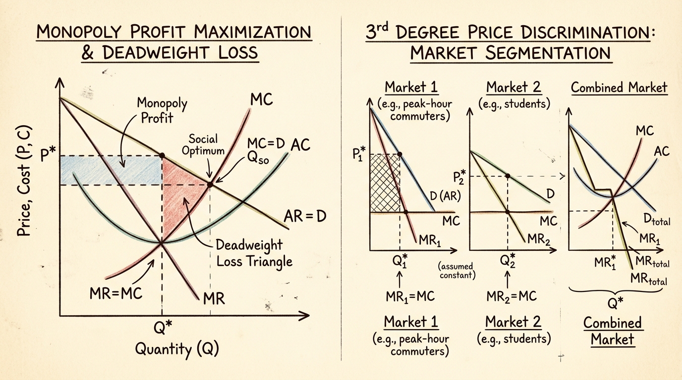
For undergraduate economics students at Delhi University, Unit 6: Monopoly and Price Discrimination marks a pivotal transition. After spending weeks mastering the theoretical utopia of perfect competition, you are now introduced to the strategic realities of market power. While perfect competition assumes firms are price-takers, this unit introduces the price-maker.
A monopoly is a market structure characterized by a single seller of a unique product with no close substitutes, protected by significant barriers to entry. In this comprehensive 3,000+ word study guide, we will unpack the core mechanics of monopoly behavior, the welfare implications (deadweight loss), and the fascinating mathematics of price discrimination. We have also included eight fully solved numerical problems mapping directly to the 15-mark DU examination format.
1. Monopoly Sources & Characteristics
Why do monopolies exist? The defining feature of a monopoly is barriers to entry. Without these barriers, positive economic profits would attract new entrants, eroding the monopolist's market power. The primary sources of monopoly power include:
- Natural Monopoly: Arises when economies of scale are so pervasive that a single firm can supply the entire market at a lower Average Total Cost (ATC) than two or more firms. Examples include local utility companies (water, electricity grids).
- Patents and Copyrights: Government-granted exclusive rights to produce or sell an invention, incentivizing innovation (e.g., pharmaceutical drugs).
- Network Externalities: A situation where the value of a product increases as more people use it, naturally leading to market dominance (e.g., social media platforms, operating systems).
- Control of Raw Materials: Exclusive ownership of a scarce resource (e.g., De Beers' historical control over the global diamond supply).
Key Characteristics
Unlike a perfectly competitive firm facing a perfectly elastic (horizontal) demand curve, a monopolist faces the downward-sloping market demand curve. This fundamentally alters their revenue structure. They cannot simply sell infinite quantities at the going market price; to sell more, they must lower the price.
2. Average & Marginal Revenue under Monopoly
For a monopolist, Average Revenue (AR) is simply the price of the good (AR = TR/Q = P(Q)). Since the demand curve is downward sloping, the AR curve is identical to the market demand curve.
Proof that MR < P
Marginal Revenue (MR) is the addition to total revenue from selling one more unit. Because the monopolist must lower the price on all units to sell an additional unit, MR is always less than the price (except at the very first unit).
Let Demand be P = a - bQ.
Total Revenue (TR) = P * Q = (a - bQ)Q = aQ - bQ^2.
Marginal Revenue (MR) = d(TR)/dQ = a - 2bQ.
Notice that the MR curve has the same price intercept (a) but twice the slope (-2b) of the demand curve. Therefore, for any Q > 0, MR < P.
Derivation of MR = P(1 - 1/|e|)
One of the most important formulas in microeconomics links Marginal Revenue to the price elasticity of demand (e).
TR = P(Q) * Q
Using the product rule: MR = d(TR)/dQ = P + Q * (dP/dQ)
Factor out P: MR = P [1 + (Q/P) * (dP/dQ)]
Recall that the price elasticity of demand is e = (dQ/dP) * (P/Q). Therefore, the reciprocal is 1/e = (dP/dQ) * (Q/P).
Substitute this back: MR = P [1 + 1/e].
Since demand elasticity (e) is negative, we can use absolute value |e|: MR = P(1 - 1/|e|).
Why a Monopolist Never Operates on the Inelastic Portion of Demand
Examine the formula MR = P(1 - 1/|e|):
- If demand is elastic (|e| > 1), 1/|e| < 1, so MR > 0.
- If demand is unit elastic (|e| = 1), 1/|e| = 1, so MR = 0.
- If demand is inelastic (|e| < 1), 1/|e| > 1, so MR < 0.
A profit-maximizing monopolist sets MR = MC. Since Marginal Cost (MC) must be positive, MR must also be positive. Therefore, a monopolist will always price on the elastic portion of the demand curve (|e| > 1). If they were on the inelastic portion, they could raise the price, which would reduce quantity, reduce total costs, but actually increase total revenue, strictly increasing profit.
3. Short-Run and Long-Run Monopoly Equilibrium
First-Order and Second-Order Conditions (FOC & SOC)
The objective of the monopolist is to maximize profit (Pi).
Pi = TR(Q) - TC(Q)
First-Order Condition (FOC): Set the first derivative to zero.
d(Pi)/dQ = d(TR)/dQ - d(TC)/dQ = 0
MR - MC = 0 => MR = MC
Second-Order Condition (SOC): The second derivative must be negative for a maximum.
d^2(Pi)/dQ^2 < 0
d(MR)/dQ - d(MC)/dQ < 0
Slope of MR < Slope of MC. This means the MC curve must cut the MR curve from below.
The Absence of a Unique Supply Curve
A frequent DU exam question asks: "Why does a monopoly not have a supply curve?"
In perfect competition, the supply curve maps Price to Quantity Supplied (because P = MC). A monopolist, however, does not take price as given. Instead, they choose output where MR = MC, and then read the price off the demand curve. Depending on the shape and elasticity of the demand curve, a monopolist could supply:
- The same quantity at two different prices (if demand curves pivot).
- Different quantities at the exact same price (if demand curves shift in specific ways).
Because there is no one-to-one relationship between Price and Quantity Supplied, a monopoly has no unique supply curve.
4. Measurement of Monopoly Power
Monopoly power is the ability of a firm to price above marginal cost. The two standard metrics are:
1. The Lerner Index (L)
The Lerner Index directly measures the markup of price over marginal cost.
L = (P - MC) / P
We can relate this to elasticity using the MR = MC equilibrium condition.
Since MR = P(1 - 1/|e|) and MR = MC:
MC = P - P/|e|
P - MC = P/|e|
(P - MC) / P = 1 / |e|
Therefore, L = 1 / |e|.
The index ranges from 0 to 1. In perfect competition, |e| is infinite, L = 0 (no market power). As demand becomes less elastic, L approaches 1, indicating high monopoly power.
2. Herfindahl-Hirschman Index (HHI)
Used by regulators to measure market concentration, the HHI is the sum of the squares of the market shares (s) of all firms in the industry.
HHI = s1^2 + s2^2 + ... + sn^2.
For a pure monopoly, s1 = 100, so HHI = 100^2 = 10,000.
5. Welfare Analysis & Social Cost of Monopoly
The Deadweight Loss (DWL) Triangle
Monopolies are inefficient compared to perfectly competitive markets. A competitive market produces where P = MC, maximizing total economic surplus. A monopolist restricts output (Qm < Qc) to raise the price (Pm > Pc).
Because P > MC for the units between Qm and Qc, consumers value these goods more than it costs to produce them. By not producing these units, the monopolist creates a Deadweight Loss (DWL)—a permanent loss of social welfare. On a graph, this is the triangle bounded by the Demand curve, the MC curve, and the monopoly output quantity Qm.
Rent-Seeking Expenditures
The true social cost of a monopoly is often higher than just the DWL triangle. Monopolists may spend vast resources (lobbying, legal fees, massive advertising) to acquire or maintain their monopoly status. These unproductive expenses are known as rent-seeking expenditures, further reducing total societal welfare.
6. Price Discrimination
Price discrimination occurs when a firm charges different prices to different consumers for the same good, where price differences are not justified by cost differences.
Required Conditions:
- The firm must have market power (price-making ability).
- The firm must be able to segment the market based on willingness to pay.
- There must be no arbitrage (consumers buying at a low price cannot resell to high-price consumers).
First-Degree (Perfect) Price Discrimination
The monopolist charges every consumer their exact maximum willingness to pay (reservation price) for each unit.Welfare Impact: The monopolist extracts 100% of the Consumer Surplus. However, because they produce every unit where P >= MC, output equals the competitive output (Qc). Deadweight Loss is ZERO. It is perfectly efficient, but perfectly inequitable.
Second-Degree Price Discrimination (Block Pricing)
The firm cannot identify individual willingness to pay, so it offers pricing menus or quantity discounts, forcing consumers to self-select. Example: Electricity blocks (first 100 units at Rs. 4/unit, next 100 at Rs. 3/unit).
Third-Degree Price Discrimination (Market Segmentation)
The most common form. The firm separates consumers into distinct markets (e.g., student vs. adult movie tickets) with different demand elasticities.
Optimization Rule: The firm maximizes profit by equating the Marginal Revenue in each market to the overall Marginal Cost.
MR1 = MR2 = MC
Since MR1 = P1(1 - 1/|e1|) and MR2 = P2(1 - 1/|e2|), equating them gives the pricing formula:
P1 / P2 = (1 - 1/|e2|) / (1 - 1/|e1|)
Rule of thumb: The sub-market with the more inelastic demand (lower |e|) will be charged the higher price.
Peak-Load Pricing
Distinct from 3rd-degree discrimination because marginal costs actually vary. Demand is higher during peak times (e.g., rush hour metro, daytime electricity). The firm charges higher prices during peak times because MC is higher (pushing against capacity constraints) and demand is more inelastic.
7. Natural Monopoly Regulation
A natural monopoly has continuously declining Average Total Cost (ATC) due to massive fixed costs. Marginal Cost (MC) is always below ATC.
- Marginal Cost Pricing (P = MC): Regulators force the firm to price at MC to achieve allocative efficiency (zero DWL). However, since MC < ATC, the firm makes an economic loss and will exit the market unless the government provides a subsidy equal to the loss.
- Average Cost Pricing (P = ATC): The regulator sets price where the demand curve intersects the ATC curve. The firm earns exactly zero economic profit (a "fair rate of return"). There is some deadweight loss, but no government subsidy is required. This is the most common regulatory compromise.
8. Fully Solved Numerical Problems (DU Exam Focus)
The backbone of DU Microeconomics exams is the numerical section. Let's walk through 8 rigorous examples.
Problem 1: Standard Monopoly Equilibrium
Q: A monopolist faces demand P = 100 - 2Q. Their total cost is TC = Q^2 + 20Q + 50. Find profit-maximizing Price, Quantity, and Profit.
Solution:
1. Find MR: TR = (100 - 2Q)Q = 100Q - 2Q^2. MR = d(TR)/dQ = 100 - 4Q.
2. Find MC: MC = d(TC)/dQ = 2Q + 20.
3. Equate MR = MC: 100 - 4Q = 2Q + 20 => 80 = 6Q => Q = 13.33 units.
4. Find Price: P = 100 - 2(13.33) = 100 - 26.67 = Rs. 73.33.
5. Find Profit: TR = 73.33 * 13.33 = 977.77. TC = (13.33)^2 + 20(13.33) + 50 = 177.77 + 266.67 + 50 = 494.44. Profit = 977.77 - 494.44 = Rs. 483.33.
Problem 2: Deadweight Loss Calculation
Q: From Problem 1, calculate the Deadweight Loss.
Solution:
1. Find Competitive Equilibrium (P = MC).
100 - 2Q = 2Q + 20 => 80 = 4Q => Qc = 20. Pc = 100 - 40 = Rs. 60.
2. Identify Monopoly variables: Qm = 13.33, Pm = 73.33. MC at Qm = 2(13.33) + 20 = 46.67.
3. Calculate DWL Area = 0.5 * Base * Height.
Base (Quantity difference) = Qc - Qm = 20 - 13.33 = 6.67.
Height (Price minus MC at Qm) = Pm - MC(Qm) = 73.33 - 46.67 = 26.66.
DWL = 0.5 * 6.67 * 26.66 = 88.91.
Problem 3: Lerner Index
Q: A monopolist has MC = Rs. 40. Demand elasticity is -3. What price should they charge? What is the Lerner Index?
Solution:
1. Use formula: MR = P(1 - 1/|e|).
2. MR = MC, so 40 = P(1 - 1/3) = P(2/3).
3. P = 40 * (3/2) = Rs. 60.
4. Lerner Index = (P - MC)/P = (60 - 40)/60 = 20/60 = 0.33 (or 1/|e| = 1/3 = 0.33).
Problem 4: Third-Degree Price Discrimination
Q: A monopolist sells in Market 1 (P1 = 50 - Q1) and Market 2 (P2 = 90 - 2Q2). Total Cost is TC = 10Q + 20, where Q = Q1 + Q2. Find Q1, P1, Q2, P2.
Solution:
1. Find MR1 and MR2: MR1 = 50 - 2Q1. MR2 = 90 - 4Q2.
2. Find MC: MC = 10.
3. Set MR1 = MC: 50 - 2Q1 = 10 => 40 = 2Q1 => Q1 = 20.
P1 = 50 - 20 = Rs. 30.
4. Set MR2 = MC: 90 - 4Q2 = 10 => 80 = 4Q2 => Q2 = 20.
P2 = 90 - 2(20) = Rs. 50.
Problem 5: Elasticity and Price Discrimination
Q: From Problem 4, calculate elasticity in both markets and verify the rule that the market with lower elasticity gets the higher price.
Solution:
e1 = (dQ1/dP1) * (P1/Q1). Since P1 = 50 - Q1, Q1 = 50 - P1, so dQ1/dP1 = -1.
|e1| = |-1| * (30/20) = 1.5.
e2 = (dQ2/dP2) * (P2/Q2). Since P2 = 90 - 2Q2, Q2 = 45 - 0.5P2, so dQ2/dP2 = -0.5.
|e2| = |-0.5| * (50/20) = 1.25.
Since 1.25 < 1.5, Market 2 has less elastic demand, which perfectly aligns with the firm charging a higher price (Rs. 50 > Rs. 30) in Market 2.
Problem 6: Multi-plant Monopoly
Q: A monopolist produces a single product in two plants. Demand: P = 120 - 3Q (where Q = Q1 + Q2). Cost Plant 1: C1 = 10Q1 + 2Q1^2. Cost Plant 2: C2 = 60Q2 + Q2^2. Find optimal output in each plant.
Solution:
Rule: MR = MC1 = MC2.
1. MR = 120 - 6Q = 120 - 6(Q1 + Q2).
2. MC1 = 10 + 4Q1.
3. MC2 = 60 + 2Q2.
Set MC1 = MC2: 10 + 4Q1 = 60 + 2Q2 => 2Q2 = 4Q1 - 50 => Q2 = 2Q1 - 25.
Set MR = MC1: 120 - 6Q1 - 6(2Q1 - 25) = 10 + 4Q1
120 - 6Q1 - 12Q1 + 150 = 10 + 4Q1
270 - 18Q1 = 10 + 4Q1
260 = 22Q1 => Q1 = 11.82.
Q2 = 2(11.82) - 25 = 23.64 - 25 = -1.36.
Crucial observation: Quantity cannot be negative! The firm will shut down Plant 2 and produce everything in Plant 1. Therefore, Q2 = 0.
Recalculate with only Plant 1: 120 - 6Q1 = 10 + 4Q1 => 110 = 10Q1 => Q1 = 11, Q2 = 0.
Problem 7: First Degree Price Discrimination
Q: A monopolist with Demand P = 100 - Q and MC = 20 practices perfect (1st degree) price discrimination. Find their total profit.
Solution:
1. Output is where P = MC: 100 - Q = 20 => Q = 80.
2. Total Revenue is the entire area under the demand curve up to Q=80.
TR = Area of trapezoid = 0.5 * (100 + 20) * 80 = 0.5 * 120 * 80 = 4,800.
3. Total Variable Cost (since MC is constant) = MC * Q = 20 * 80 = 1,600.
4. Profit (ignoring fixed cost) = 4,800 - 1,600 = 3,200.
Notice this equals the entire Consumer Surplus + Producer Surplus of a competitive market.
Problem 8: Natural Monopoly Regulation
Q: Natural Monopoly faces Demand P = 50 - Q. TC = 100 + 10Q. Compare MC pricing and ATC pricing.
Solution:
MC = 10. ATC = 100/Q + 10.
Case 1: MC Pricing (Allocative Efficiency)
Set P = MC: 50 - Q = 10 => Q = 40. P = 10.
Profit = TR - TC = (10*40) - (100 + 10(40)) = 400 - 500 = -100.
The firm loses 100 and requires a government subsidy.
Case 2: Average Cost Pricing (Fair Rate of Return)
Set P = ATC: 50 - Q = 100/Q + 10
40 - Q = 100/Q => 40Q - Q^2 = 100 => Q^2 - 40Q + 100 = 0.
Using quadratic formula: Q = [40 +/- sqrt(1600 - 400)] / 2 = [40 +/- 34.64]/2.
Q = 37.32 (since we want the larger output for regulation).
P = 50 - 37.32 = 12.68.
Profit = TR - TC = (12.68 * 37.32) - (100 + 10*37.32) = 473 - 473 = 0.
Firm breaks even, no subsidy required, but output is slightly less than efficient Q=40.
9. DU Exam Blueprint & Model 15-Mark Solutions
How Unit 6 is Tested
Unit 6 generally accounts for 20-25% of your final exam weight. You will almost certainly see a 15-mark composite question structured like this:
- Part A (5 Marks): Theory/Proof. "Prove that a monopolist will never operate on the inelastic portion of the demand curve" or "Explain the concept of Deadweight Loss using a diagram."
- Part B (10 Marks): Numerical. Usually Third-Degree Price Discrimination across two markets, asking you to calculate P, Q, and Profit under discrimination vs. non-discrimination, and prove the elasticities.
Exam Tips to Maximize Marks
- Always Draw the Diagram: In any theory question about monopoly equilibrium, DWL, or price discrimination, a well-labeled graph is worth 2-3 explicit marks. Label axes (Price/Cost vs Quantity), mark MR, AR, MC, and clearly shade the DWL or Profit boxes.
- Second Order Conditions: In numerical problems, after finding MR = MC, add a quick line: "Check SOC: Slope of MR (-4) < Slope of MC (2). Condition satisfied." Examiners look for this explicitly for the final out-of-10 mark.
- Formulas First: Don't just crunch numbers. Write MR = P(1 - 1/|e|) before plugging in values. State the profit-maximizing rule clearly before solving equations.
- Check for Corner Solutions: As seen in Problem 6, if your math yields a negative quantity for a market or plant, state that output cannot be negative and set it to zero, recalculating for the active market.
Mastering monopoly and price discrimination gives you the algebraic and geometric intuition needed for everything that follows in intermediate microeconomics, especially oligopoly and game theory. Drill the numericals until the MR=MC rule becomes second nature. Good luck with your preparation!
Frequently asked questions
Why is MR less than P for a monopolist?
Because to sell an additional unit, the monopolist must lower the price on all prior units sold, pushing Marginal Revenue below the price.
What is 3rd degree price discrimination?
Charging different prices in different sub-markets based on their price elasticities, using the rule MR1 = MR2 = MC.
Dhairya sat the same DU papers he now writes about. Acadly is his attempt to say the useful things his own first-year self would have wanted to hear.
Keep reading
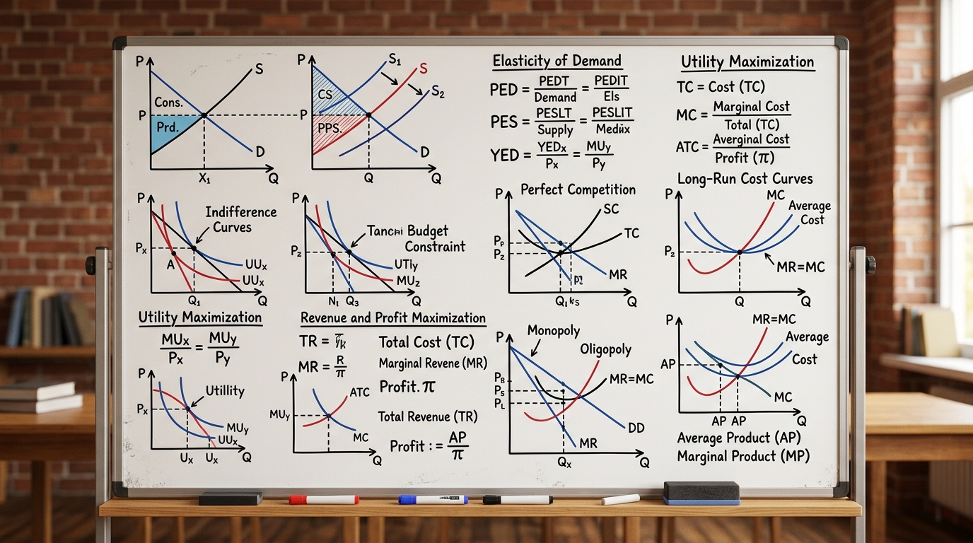
Microeconomics Formula Sheet & Key Theorems: The Complete DU Reference Guide
The ultimate cheat sheet for Intermediate Microeconomics I & II. Master Consumer Theory, Producer Theory, Market Structures, Game Theory, and Welfare Economics.
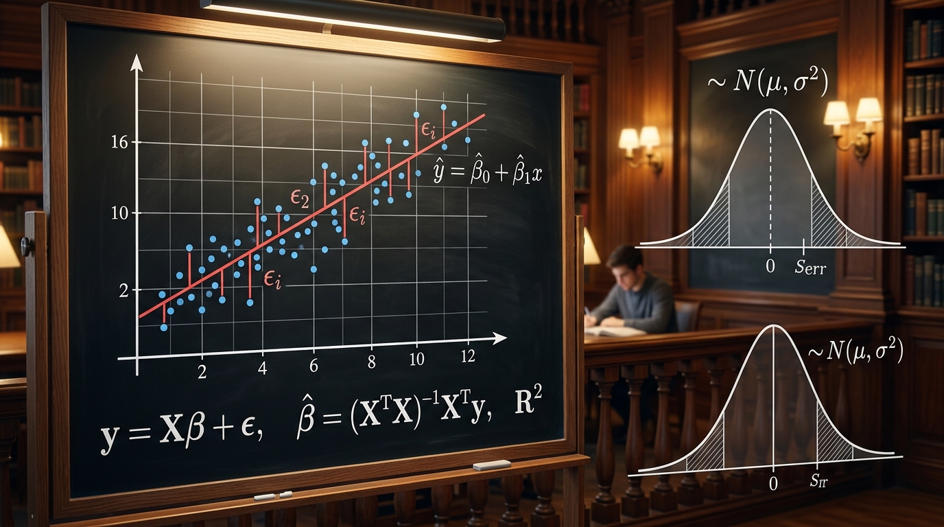
Introductory Econometrics & OLS Regression: Gauss-Markov Theorem, Proofs & Exam Numericals
Comprehensive 4,500-word masterclass on Introductory Econometrics and Ordinary Least Squares (OLS) for DU Economics students. Covers algebraic derivations of beta_0 and beta_1, Gauss-Markov BLUE proofs, R-squared variance decomposition, hypothesis testing (t and F-tests), and 3 fully worked numerical problems.
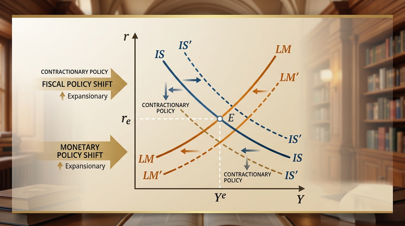
IS-LM Model: Goods & Money Market Equilibrium, Policy Multipliers & DU Exam Numericals
Comprehensive 4,000-word masterclass on the IS-LM model for DU Economics students. Covers algebraic derivations of IS and LM curves, general equilibrium, fiscal and monetary policy multipliers, crowding-out effect, liquidity trap, and 3 fully worked exam numericals.