Introductory Microeconomics Unit 8: Factor Markets, Labor Demand-Supply & Economic Rent Notes
Master DU Sem 1 Unit 8: Derived demand for labor, VMPL vs MRPL, backward-bending labor supply, monopsony exploitation & Ricardian/modern economic rent.
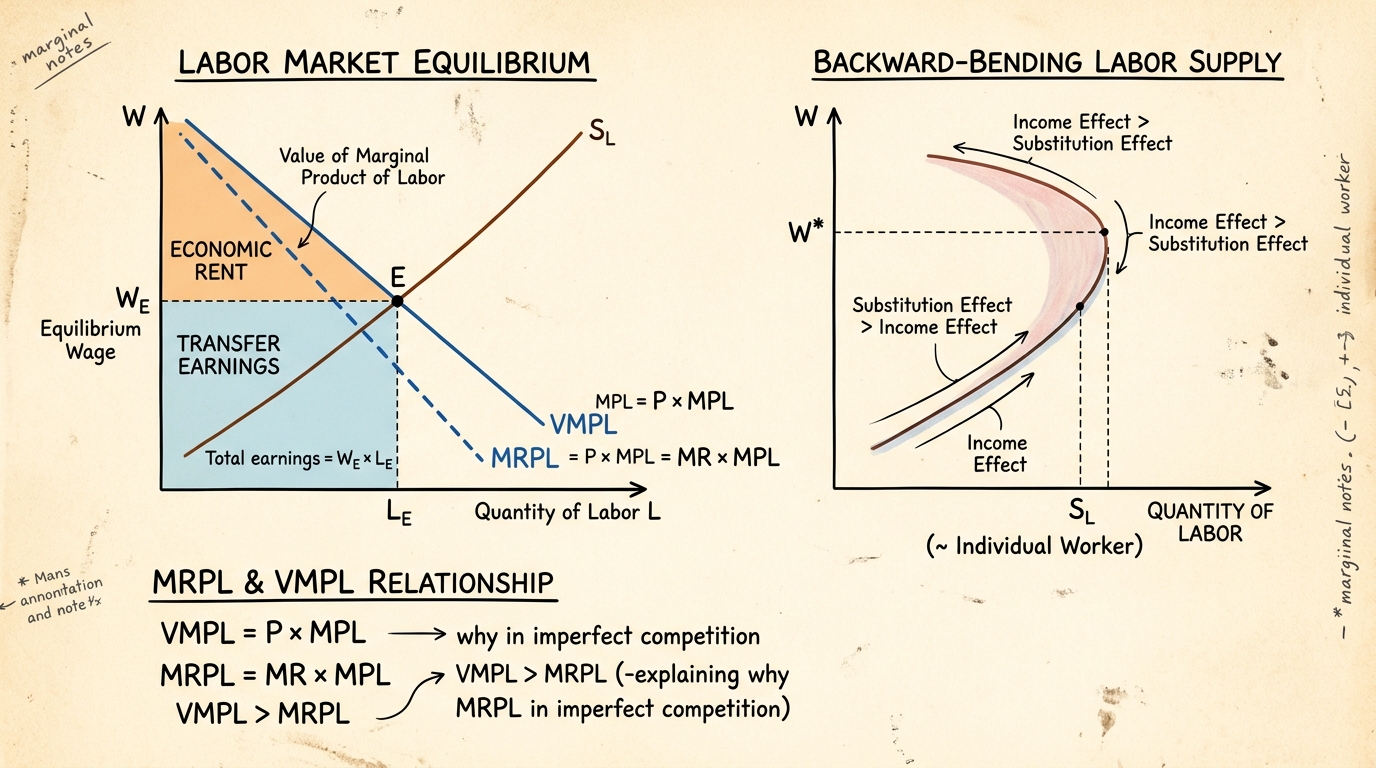
Welcome to the most comprehensive study guide for Unit 8: Factor Markets, Labor Supply, and Economic Rent for Delhi University’s BA (Hons) Economics Semester 1 Introductory Microeconomics paper. While units like consumer theory and market structures look at the product market (where firms sell goods to consumers), this unit flips the script. Now we are looking at the factor market—where households supply factors of production (like labor, land, and capital) and firms demand them.
This unit is heavily mathematical but also deeply intuitive. We will explore how wages are determined, why people might choose to work less when their wages rise too high (the backward-bending labor supply curve), what happens when a single firm dominates the labor market (monopsony), and the concept of economic rent. Historically, DU examiners love testing numericals on VMPL (Value of Marginal Product of Labor) and MRPL (Marginal Revenue Product of Labor), along with theoretical essays on the income and substitution effects of a wage change.
In this 3,000+ word guide, we will break down every concept step-by-step, accompanied by 8 fully solved numerical problems mirroring past year questions (PYQs) and a dedicated section on exam strategy. Let’s dive in.
1. Factor Demand as Derived Demand
The defining feature of the demand for any factor of production is that it is a derived demand. A firm does not demand labor just for the sake of having employees; it demands labor because it needs to produce output that consumers want to buy. If the demand for the final product falls, the demand for the labor used to make it will also fall.
Marginal Product of Labor (MPL)
The Marginal Product of Labor (MPL) is the additional output a firm produces by hiring one more unit of labor, holding all other inputs (like capital) constant. Mathematically, it is the derivative of the production function with respect to labor: MPL = dQ/dL. Due to the Law of Diminishing Marginal Returns, MPL eventually declines as more labor is hired.
Value of Marginal Product (VMPL)
If the firm is operating in a perfectly competitive product market, it can sell all the output it wants at the prevailing market price P. The monetary value of the extra output produced by one more worker is called the Value of Marginal Product of Labor (VMPL).
Formula: VMPL = P * MPL
VMPL represents the firm's demand curve for labor in a perfectly competitive product market. Because MPL is downward sloping (diminishing returns), the VMPL curve is also downward sloping.
Marginal Revenue Product (MRPL)
What if the firm is a monopolist in the product market? To sell more output, it must lower its price. Therefore, the extra revenue generated by one more worker is not just P * MPL. Instead, we use Marginal Revenue (MR). The Marginal Revenue Product of Labor (MRPL) is the extra revenue generated by hiring one more unit of labor.
Formula: MRPL = MR * MPL
For a perfectly competitive firm, P = MR, so VMPL = MRPL. But for a monopolist, MR is less than P, so MRPL is less than VMPL. The firm’s demand curve for labor is always its MRPL curve.
2. Profit-Maximizing Demand for Input
How does a firm decide exactly how many workers to hire? It uses marginal analysis. The extra revenue from hiring a worker is VMPL (or MRPL). The extra cost of hiring that worker is the wage rate, w (assuming a competitive labor market where the firm is a wage taker).
The Golden Rule of Hiring
A profit-maximizing firm will continue to hire labor as long as the additional revenue from the worker exceeds the additional cost. The firm stops hiring exactly where the marginal benefit equals the marginal cost.
For a firm in a competitive product market: Hire until VMPL = w (or P * MPL = w).
For a monopolist in the product market: Hire until MRPL = w (or MR * MPL = w).
Hicks-Marshall Laws of Derived Factor Demand
The Hicks-Marshall laws explain the factors that determine the elasticity of demand for a factor of production (e.g., how sensitive a firm's demand for labor is to a change in wages). The demand for labor will be more elastic when:
- High elasticity of product demand: If consumers are very sensitive to the price of the final good, then an increase in wages (which raises the good's price) will lead to a massive drop in product sales, and thus a massive drop in labor demand.
- Easy substitutability of other factors: If machines can easily replace humans, a small wage hike will cause firms to rapidly switch to capital, making labor demand highly elastic.
- High supply elasticity of other factors: If the price of capital (machines) doesn't shoot up when firms try to substitute labor with capital, firms will easily switch, making labor demand elastic.
- Large share of total cost: If labor costs make up 90% of a firm's total costs, a wage increase has a huge impact on total costs, making the firm highly responsive (elastic demand).
3. Supply of Labor: The Labor-Leisure Trade-Off
Unlike firms, which maximize profits, workers (households) maximize utility. They face a trade-off between income (which buys consumption goods) and leisure (free time). Working more means more income but less leisure.
Indifference Curves and Budget Constraint
We can model this using consumer theory. The worker has a total time endowment, say T hours (e.g., 24 hours a day). Let L be hours worked and R be hours of leisure. So, T = L + R.
Income (Y) is earned by working at wage w: Y = w * L = w * (T - R).
The worker's utility function is U(Y, R). The indifference curves represent combinations of income and leisure that give the same level of satisfaction. The budget constraint is the straight line representing the maximum income achievable for any given amount of leisure, with a slope of -w (the opportunity cost of leisure is the wage).
Equilibrium occurs where the highest indifference curve is tangent to the budget constraint. At this point, the Marginal Rate of Substitution between leisure and income (MRS) equals the wage rate w.
Income vs. Substitution Effect of a Wage Increase
When the wage rate w increases, what happens to the hours of labor supplied? It depends on two opposing effects:
- Substitution Effect (SE): As the wage rises, leisure becomes more expensive (higher opportunity cost). The worker substitutes away from leisure towards work. SE always increases labor supply.
- Income Effect (IE): As the wage rises, the worker is effectively richer for the same hours worked. Since leisure is a normal good, a richer person wants to consume more of it. IE always decreases labor supply.
The Backward-Bending Labor Supply Curve
At lower wage levels, the Substitution Effect dominates the Income Effect (SE > IE). An increase in wages leads to more hours worked. The labor supply curve is upward sloping.
However, at very high wage levels, the worker is already earning a substantial amount. The Income Effect begins to dominate the Substitution Effect (IE > SE). A further increase in wages makes the worker feel wealthy enough to "buy" more leisure, and they actually reduce the hours they work. The labor supply curve bends backward! This is a classic DU essay topic.
4. Competitive Factor Market Equilibrium
In a perfectly competitive labor market, there are many identical workers and many identical firms. No single firm or worker can influence the wage. The market wage (w) is determined by the intersection of the market demand for labor (the horizontal sum of all firms' VMPL curves) and the market supply of labor.
At equilibrium, w = VMPL. The market clears, meaning there is no involuntary unemployment (everyone willing to work at the equilibrium wage finds a job). The total employment level is L*.
5. Imperfect Factor Markets: Monopsony & Product Monopoly
Real-world labor markets are rarely perfectly competitive. Let's look at two major imperfections.
Product Market Monopoly (MRPL < VMPL)
If a firm is the sole seller in the product market but buys labor in a competitive labor market, it still faces a constant wage w. However, its labor demand curve is its MRPL curve, not VMPL. Because MR < P for a monopolist, MRPL < VMPL.
The firm hires where MRPL = w. Since MRPL is below VMPL, a monopolist hires fewer workers than a perfectly competitive industry would. This is one reason monopolies lead to lower employment in their respective sectors.
Monopsony in the Labor Market
A Monopsony is a market with only one buyer. In a labor context, it is a single employer in a town (like a coal mine in a remote village).
Because the monopsonist is the entire market demand for labor, it faces the upward-sloping market supply curve of labor. If it wants to hire more workers, it must raise the wage not just for the new worker, but for all existing workers!
This means the Marginal Factor Cost (MFC) (or Marginal Expense of Labor) is greater than the wage w.
Profit Maximization for a Monopsonist:The firm hires labor up to the point where MRPL = MFC. (Or VMPL = MFC if the product market is competitive).
At this quantity of labor (Lm), the firm looks at the labor supply curve to see the minimum wage (wm) it needs to pay to attract that many workers.
Monopsonistic Exploitation
Under monopsony, the wage paid to the worker (wm) is strictly less than their contribution to the firm's revenue (VMPL or MRPL). The difference, VMPL - wm, is called monopsonistic exploitation. The firm restricts employment to drive down wages and increase its profits.
Minimum Wage Legislation in a Monopsony
In a perfectly competitive labor market, a binding minimum wage above the equilibrium wage causes unemployment. But in a monopsony, a carefully set minimum wage can actually increase both wages and employment!
By enforcing a minimum wage, the government makes the MFC curve horizontal (equal to the minimum wage) up to the supply curve. The monopsonist no longer has to raise wages for everyone to hire one more worker. It simply hires where VMPL equals the minimum wage, leading to higher employment and ending the exploitation.
6. Theories of Factor Rewards & Economic Rent
How are factors rewarded, and what exactly is "rent" in economics? Let's unpack the classical and modern theories.
Ricardian Theory of Differential Rent
David Ricardo originally formulated the theory of rent concerning land. He argued that rent arises because land is heterogeneous in fertility and fixed in supply.
When population is small, only the most fertile (Grade A) land is cultivated. As population grows, demand for food rises, and less fertile (Grade B) land must be used. To make Grade B land profitable, the price of corn must be high enough to cover its costs.
At this higher price, the farmers on Grade A land are now making a surplus above their costs. This surplus is differential rent. The marginal land (Grade B) pays no rent. Rent is price-determined, not price-determining (high corn prices cause high rent, high rent doesn't cause high corn prices).
Modern Concept of Economic Rent
Modern economists expanded the concept of rent to all factors of production, not just land.
Transfer Earnings: The minimum payment required to keep a factor in its current occupation. (Its opportunity cost).
Actual Earnings: What the factor actually earns in its current occupation.
Economic Rent = Actual Earnings - Transfer Earnings
Economic rent is any payment above the minimum required to keep the factor supplied.
Supply Elasticity and the Share of Rent
The proportion of total earnings that constitutes economic rent depends entirely on the elasticity of supply of the factor:
- Perfectly Elastic Supply (Horizontal): The firm can hire infinite amounts at the prevailing wage. Transfer earnings equal actual earnings. Economic rent is ZERO.
- Perfectly Inelastic Supply (Vertical): The factor supply is fixed (like land, or the unique talent of a superstar athlete). Transfer earnings are zero (they would supply the same amount even at a near-zero wage). Therefore, the ENTIRE payment is Economic Rent.
- Upward Sloping Supply: Typical labor market. The area under the wage line but above the supply curve represents the total Economic Rent earned by workers.
Marshallian Quasi-Rent
Alfred Marshall introduced "Quasi-Rent" to describe surplus earnings of man-made capital equipment in the short run.
In the short run, capital (like a factory machine) is fixed in supply. Its return resembles land rent. If demand for the product rises, the earnings of the machine spike. This temporary surplus is Quasi-Rent.
Formula: Quasi-Rent = Total Revenue - Total Variable Cost.
In the long run, supply of capital is perfectly elastic (more machines can be built), so Quasi-Rent disappears.
7. 8+ Fully Solved Numerical Problems
The DU semester exam will undoubtedly feature numericals on factor markets. Here are 8 solved examples covering the full spectrum of difficulty.
Problem 1: Perfect Competition Profit Maximization
Q: A firm sells its product in a perfectly competitive market at P = $10. Its production function is Q = 50L - 2L^2. The labor market is perfectly competitive, and the wage rate is w = $100. Find the profit-maximizing level of labor (L*).
Solution:
Step 1: Find Marginal Product of Labor (MPL).
MPL = dQ/dL = 50 - 4L.
Step 2: Find Value of Marginal Product (VMPL).
VMPL = P * MPL = 10 * (50 - 4L) = 500 - 40L.
Step 3: Apply the profit-maximizing condition VMPL = w.
500 - 40L = 100
400 = 40L
L* = 10.
Answer: The firm hires 10 workers.
Problem 2: Product Market Monopoly
Q: A monopolist faces the demand curve P = 100 - 2Q. Its production function is simply Q = 5L. The wage rate is fixed at w = 100. How much labor should the monopolist hire?
Solution:
Step 1: Express Total Revenue (TR) in terms of L.
First, express TR in terms of Q: TR = P * Q = (100 - 2Q) * Q = 100Q - 2Q^2.
Now substitute Q = 5L: TR = 100(5L) - 2(5L)^2 = 500L - 2(25L^2) = 500L - 50L^2.
Step 2: Find Marginal Revenue Product of Labor (MRPL).
MRPL = d(TR)/dL = 500 - 100L.
Step 3: Set MRPL = w.
500 - 100L = 100
400 = 100L
L* = 4.
Answer: The monopolist hires 4 workers.
Problem 3: Monopsony Labor Market
Q: A firm is a monopsonist in the labor market. The supply curve for labor is L = w - 10, which means the wage function is w = L + 10. The firm’s MRPL is MRPL = 50 - 2L. Find the equilibrium wage and quantity of labor.
Solution:
Step 1: Find Total Factor Cost (TFC).
TFC = w * L = (L + 10) * L = L^2 + 10L.
Step 2: Find Marginal Factor Cost (MFC).
MFC = d(TFC)/dL = 2L + 10.
Step 3: Set MRPL = MFC to find L*.
50 - 2L = 2L + 10
40 = 4L
L* = 10.
Step 4: Find the wage the monopsonist pays (plug L* into the supply curve, NOT the MFC or MRPL).
w* = L* + 10 = 10 + 10 = 20.
Answer: Labor hired is 10 units at a wage of $20. (Notice MFC at L=10 is 30, which is higher than the wage 20. Monopsonistic exploitation is MRPL - w = 30 - 20 = $10 per worker).
Problem 4: Calculating Economic Rent from Supply Curve
Q: The market supply of specialized IT consultants is given by L = 2w. The market equilibrium wage is w = 500. What is the total Economic Rent earned by all consultants in the market?
Solution:
Step 1: Find equilibrium quantity L*.
L* = 2(500) = 1000.
Step 2: Rewrite supply as a wage equation (inverse supply).
w = 0.5L.
Step 3: Total Earnings = w* * L* = 500 * 1000 = 500,000.
Step 4: Transfer Earnings = Area under the supply curve up to L*.
The supply curve is a straight line from the origin. The area under it is a triangle.
Area = 0.5 * base * height = 0.5 * L* * (wage at L*) = 0.5 * 1000 * 500 = 250,000.
Step 5: Economic Rent = Total Earnings - Transfer Earnings.
Economic Rent = 500,000 - 250,000 = 250,000.
Answer: Total Economic Rent is 250,000. (Since the supply curve is linear from the origin, rent is exactly half of total earnings).
Problem 5: Minimum Wage in a Competitive Market
Q: The demand for labor is Ld = 100 - w. The supply of labor is Ls = 20 + 3w. The government imposes a minimum wage of w = 25. Calculate the unemployment created.
Solution:
Step 1: Check original equilibrium (optional but good practice).
100 - w = 20 + 3w => 80 = 4w => w = 20.
Since the minimum wage (25) is above the equilibrium (20), it is binding.
Step 2: Find labor demanded at w = 25.
Ld = 100 - 25 = 75.
Step 3: Find labor supplied at w = 25.
Ls = 20 + 3(25) = 20 + 75 = 95.
Step 4: Unemployment = Ls - Ld.
Unemployment = 95 - 75 = 20.
Answer: The minimum wage creates 20 units of unemployment.
Problem 6: Deriving Labor Supply from Utility Function
Q: A worker has 24 hours of time. Their utility function over consumption (C) and leisure (R) is U = C * R. The price of consumption is 1. Non-labor income is 0. Find the optimal hours of labor supply (L) as a function of the wage w.
Solution:
Step 1: Write the budget constraint.
C = w * L. Since L = 24 - R, C = w * (24 - R), or C + wR = 24w.
Step 2: Use the MRS = Price Ratio condition.
MRS = (Marginal Utility of R) / (Marginal Utility of C).
MU_R = dU/dR = C.
MU_C = dU/dC = R.
MRS = C / R.
Price ratio = w / 1 = w.
Set MRS = w => C / R = w => C = wR.
Step 3: Substitute back into budget constraint.
(wR) + wR = 24w
2wR = 24w
R = 12.
Step 4: Find Labor L.
L = 24 - R = 24 - 12 = 12.
Answer: The optimal labor supply is L = 12 hours. (Notice that with this specific Cobb-Douglas utility function, labor supply is independent of the wage rate! The substitution and income effects exactly cancel out).
Problem 7: Firm Profit with Fixed Capital
Q: A firm has the production function Q = K^0.5 * L^0.5. In the short run, capital is fixed at K = 100. Price of output P = 10, wage w = 5, rental rate of capital r = 10. Find the profit-maximizing L and the quasi-rent.
Solution:
Step 1: Substitute fixed K into production function.
Q = (100)^0.5 * L^0.5 = 10 * L^0.5.
Step 2: Find MPL.
MPL = dQ/dL = 10 * 0.5 * L^(-0.5) = 5 * L^(-0.5).
Step 3: Find VMPL.
VMPL = P * MPL = 10 * [5 * L^(-0.5)] = 50 * L^(-0.5).
Step 4: Set VMPL = w to find L*.
50 * L^(-0.5) = 5
L^(-0.5) = 0.1
1 / sqrt(L) = 0.1 => sqrt(L) = 10 => L* = 100.
Step 5: Calculate Quasi-Rent.
First, find Q* = 10 * (100)^0.5 = 10 * 10 = 100.
Total Revenue = P * Q = 10 * 100 = 1000.
Total Variable Cost = w * L = 5 * 100 = 500.
Quasi-Rent = TR - TVC = 1000 - 500 = 500.
(Note: Fixed cost is r*K = 10*100 = 1000. Pure profit is TR - TC = 1000 - 1500 = -500. Despite losses, the firm operates because Quasi-Rent is positive).
Answer: L* = 100, Quasi-Rent = 500.
Problem 8: Comparing Monopsony and Perfect Competition
Q: VMPL = 200 - 2L. Labor supply is w = 20 + 2L. What is the deadweight loss (welfare loss) of monopsony compared to a perfectly competitive labor market?
Solution:
Step 1: Find Competitive Equilibrium (VMPL = Supply).
200 - 2L = 20 + 2L
180 = 4L => Lc = 45.
Competitive wage wc = 20 + 2(45) = 110.
Step 2: Find Monopsony Equilibrium (VMPL = MFC).
Total Cost = w*L = (20 + 2L)*L = 20L + 2L^2.
MFC = 20 + 4L.
Set VMPL = MFC: 200 - 2L = 20 + 4L => 180 = 6L => Lm = 30.
Monopsony wage wm = 20 + 2(30) = 80.
Step 3: Calculate Deadweight Loss (DWL).
DWL is the area of the triangle between the VMPL curve and the Supply curve, from Lm to Lc.
Base of triangle = Lc - Lm = 45 - 30 = 15.
Height of triangle = VMPL at Lm - Supply at Lm.
VMPL at 30 = 200 - 2(30) = 140.
Supply at 30 = wm = 80.
Height = 140 - 80 = 60.
DWL = 0.5 * Base * Height = 0.5 * 15 * 60 = 450.
Answer: The deadweight loss caused by the monopsony is 450.
8. DU Exam Insights & Essay Blueprint
Unit 8 is a highly predictable scoring zone in the DU Semester 1 exam. Examiners generally pick one of three distinct tracks for the 15-mark long answer section. Here is the blueprint to tackle them.
Pattern 1: The Backward-Bending Supply Curve Essay (15 Marks)
This is the most famous qualitative question in labor economics. The question usually asks: "Using indifference curve analysis, explain the income and substitution effects of a wage increase. Can the labor supply curve bend backward?"
The 15-Mark Blueprint:
- Introduction (2 marks): Define the labor-leisure trade-off and state the budget constraint C = w(24 - R).
- Graph 1 - IC Analysis (4 marks): Draw the budget line and indifference curve. Show the initial equilibrium where MRS = w.
- Decomposing the Effects (5 marks): Break down a wage increase. Define the Substitution Effect (wage goes up, leisure is more expensive, work more). Define the Income Effect (wage goes up, you are richer, buy more leisure, work less). Explain how to graphically separate them using a Hicksian compensated budget line.
- The Bend (3 marks): Explicitly state that at low wages, SE > IE, so supply slopes up. At high wages, IE > SE, so supply slopes back.
- Graph 2 (1 mark): Draw the actual backward-bending labor supply curve placing Wage on the Y-axis and Hours Worked on the X-axis.
Pattern 2: The Monopsony Explainer & Numericals (10 + 5 Marks)
You will likely see a 10-mark theoretical explanation of monopsonistic exploitation followed by a 5-mark numerical (like Problem 3 above).
The Blueprint:
- Definition (2 marks): Define monopsony. Clarify that it faces an upward-sloping supply curve, meaning MFC > w.
- Graph (5 marks): This is non-negotiable. Draw VMPL (downward), Supply (upward), and MFC (upward and steeper than Supply). Mark the equilibrium quantity where VMPL = MFC, and show that the wage is read off the Supply curve, not the MFC curve.
- Exploitation (3 marks): Define Monopsonistic Exploitation as the vertical gap between VMPL and the wage paid at the equilibrium quantity. Mention Joan Robinson, the economist who formalized this.
Pattern 3: Economic Rent vs. Transfer Earnings (10 Marks)
This is a standard short-note or 10-mark question: "Distinguish between Transfer Earnings and Economic Rent. How does the elasticity of supply affect the proportion of rent?"
The Blueprint:
- Definitions (2 marks): Define transfer earnings (opportunity cost) and economic rent (surplus).
- The Formula (1 mark): Economic Rent = Actual Earnings - Transfer Earnings.
- The Three Cases (6 marks): Draw three small graphs side-by-side.
1. Horizontal supply (Perfectly elastic, Rent = 0).
2. Vertical supply (Perfectly inelastic, Rent = Total Earnings).
3. Upward sloping supply (Rent = Area above supply curve, below wage line). - Quasi-Rent (1 mark): Add a concluding sentence defining Marshallian Quasi-Rent as the short-run equivalent for man-made capital.
Common Traps to Avoid
- Confusing MRPL and VMPL: VMPL is P * MPL. MRPL is MR * MPL. They are only equal if the firm is in a perfectly competitive product market. If the question states the firm faces a downward-sloping demand curve, you MUST use MRPL to find labor demand.
- Monopsony Wage Determination: The biggest mistake students make is finding L* where MRPL = MFC, and then plugging L* back into the MFC curve to find the wage. NO! You plug L* into the Supply curve to find the wage. The firm pays the lowest wage possible to attract L* workers, which is given by the supply curve.
- Units in Numericals: Always read carefully to see if the question gives you a wage in thousands or dollars, and ensure your final interpretation matches. If asked for Deadweight Loss, remember it's an area (0.5 * base * height), not a single point.
Conclusion
Unit 8 ties together the theories of the firm and the consumer. By understanding that factor demand is derived from product demand, and that labor supply is a choice between income and leisure, you now have a complete picture of the microeconomic cycle. Master the differences between VMPL and MRPL, practice the monopsony derivations, and understand the modern definition of economic rent. With the PYQ blueprints and the 8 solved numericals above, you are more than ready to conquer the factor markets section of your DU Semester 1 Introductory Microeconomics exam. Good luck!
Frequently asked questions
What is the difference between VMPL and MRPL?
VMPL is the value of the marginal product (P * MPL) used by competitive firms. MRPL is the marginal revenue product (MR * MPL) used by monopolists.
Why does the labor supply curve bend backward?
At very high wages, workers are wealthy enough that the income effect (desire for more leisure) dominates the substitution effect (higher opportunity cost of leisure).
What is monopsonistic exploitation?
It occurs when a single buyer of labor (monopsony) pays a wage lower than the worker's marginal contribution to revenue (VMPL or MRPL).
Dhairya sat the same DU papers he now writes about. Acadly is his attempt to say the useful things his own first-year self would have wanted to hear.
Keep reading
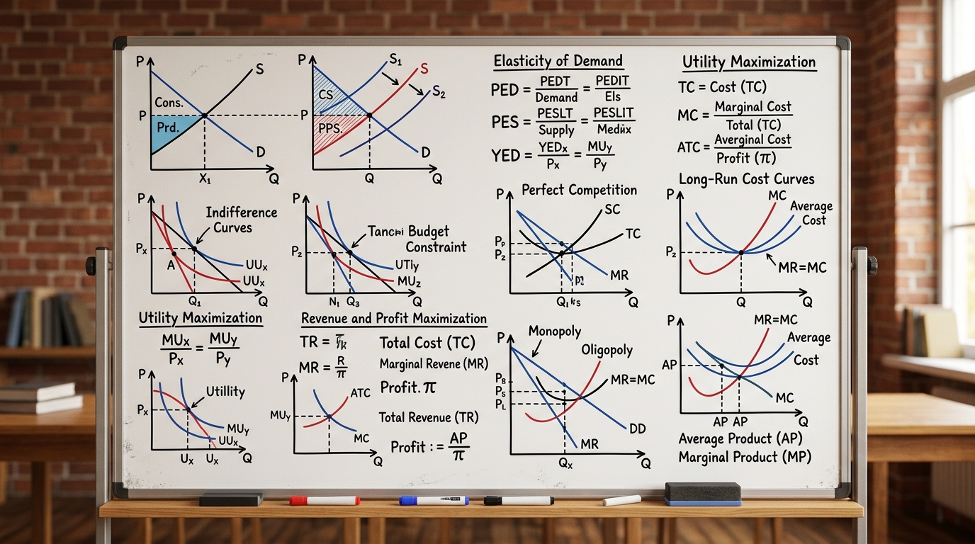
Microeconomics Formula Sheet & Key Theorems: The Complete DU Reference Guide
The ultimate cheat sheet for Intermediate Microeconomics I & II. Master Consumer Theory, Producer Theory, Market Structures, Game Theory, and Welfare Economics.

Introductory Econometrics & OLS Regression: Gauss-Markov Theorem, Proofs & Exam Numericals
Comprehensive 4,500-word masterclass on Introductory Econometrics and Ordinary Least Squares (OLS) for DU Economics students. Covers algebraic derivations of beta_0 and beta_1, Gauss-Markov BLUE proofs, R-squared variance decomposition, hypothesis testing (t and F-tests), and 3 fully worked numerical problems.
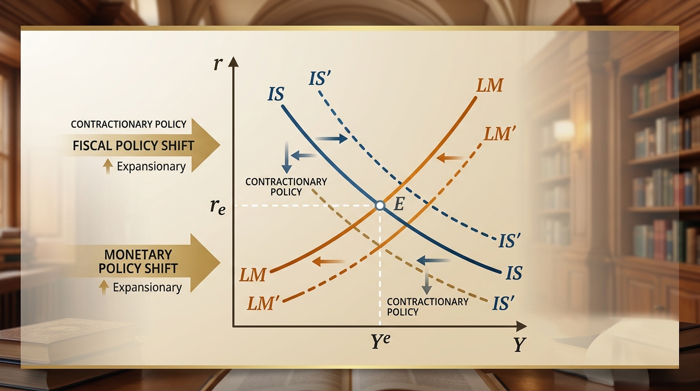
IS-LM Model: Goods & Money Market Equilibrium, Policy Multipliers & DU Exam Numericals
Comprehensive 4,000-word masterclass on the IS-LM model for DU Economics students. Covers algebraic derivations of IS and LM curves, general equilibrium, fiscal and monetary policy multipliers, crowding-out effect, liquidity trap, and 3 fully worked exam numericals.